

Abstract
Biodiversity in ecosystems plays an important role in supporting human welfare, including regulating the transmission of infectious diseases. Many of these services are not fully-appreciated due to complex environmental dynamics and lack of baseline data. Multicontinental amphibian decline due to the fungal pathogen Batrachochytrium dendrobatidis (Bd) provides a stark example. Even though amphibians are known to affect natural food webs—including mosquitoes that transmit human diseases—the human health impacts connected to their massive decline have received little attention. Here we leverage a unique ensemble of ecological surveys, satellite data, and newly digitized public health records to show an empirical link between a wave of Bd-driven collapse of amphibians in Costa Rica and Panama and increased human malaria incidence. Subsequent to the estimated date of Bd-driven amphibian decline in each 'county' (canton or distrito), we find that malaria cases are significantly elevated for several years. For the six year peak of the estimated effect, the annual expected county-level increase in malaria ranges from 0.76 to 1.1 additional cases per 1000 population. This is a substantial increase given that cases country-wide per 1000 population peaked during the timeframe of our study at approximately 1.5 for Costa Rica and 1.1 for Panama. This previously unidentified impact of biodiversity loss illustrates the often hidden human welfare costs of conservation failures. These findings also show the importance of mitigating international trade-driven spread of similar emergent pathogens like Batrachochytrium salamandrivorans.
Export citation and abstract BibTeX RIS
1. Introduction
Despite recent catastrophic, disease-driven loss of amphibians at a global scale [1], no broad implications for human welfare have been empirically demonstrated. Amphibians are not unique in this regard. While broad biodiversity loss impedes ecosystem functioning and the social benefits that follow, specific consequences of such change often go unnoticed [2]. For amphibians, the spread of Batrachochytrium dendrobatidis (Bd)—an extremely virulent fungal pathogen responsible for massive worldwide die-offs from the resulting chytridiomycosis [3]—has arguably caused 'the greatest recorded loss of biodiversity attributable to a disease' [1]. The Bd fungus disperses into its environment as motile spores (zoospores) that swim in water or over wet surfaces, which infect the skin of amphibians, disrupting key functions of their skin (like osmotic regulation) and often leading to death [3]. Empirical reckoning with implications for human welfare is essential for informed mitigation of ongoing impacts and—perhaps more importantly—sufficiently motivating investment to avoid repeating such disasters. For example, newer related pathogens like Batrachochytrium salamandrivorans similarly threaten to invade through the global movement of goods and people, repeating the cycle [4].
A global review of Bd impacts on amphibians by Scheele et al [1] attributed the extinction of at least 90 species to this pathogen. An additional 411 species (at minimum) have declined in abundance because of Bd, with over 30% of these species showing population losses exceeding 90%. The emergent approaches of both One Health and Planetary Health emphasize ties between people, animals, plants, and environment, for example human-mammal/bird connections in outbreaks of novel influenza and coronaviruses [5]. While both frameworks have been influential in promoting the connection between human and animal health [6], relatively little attention has been paid to the linkage between amphibians and human well-being.
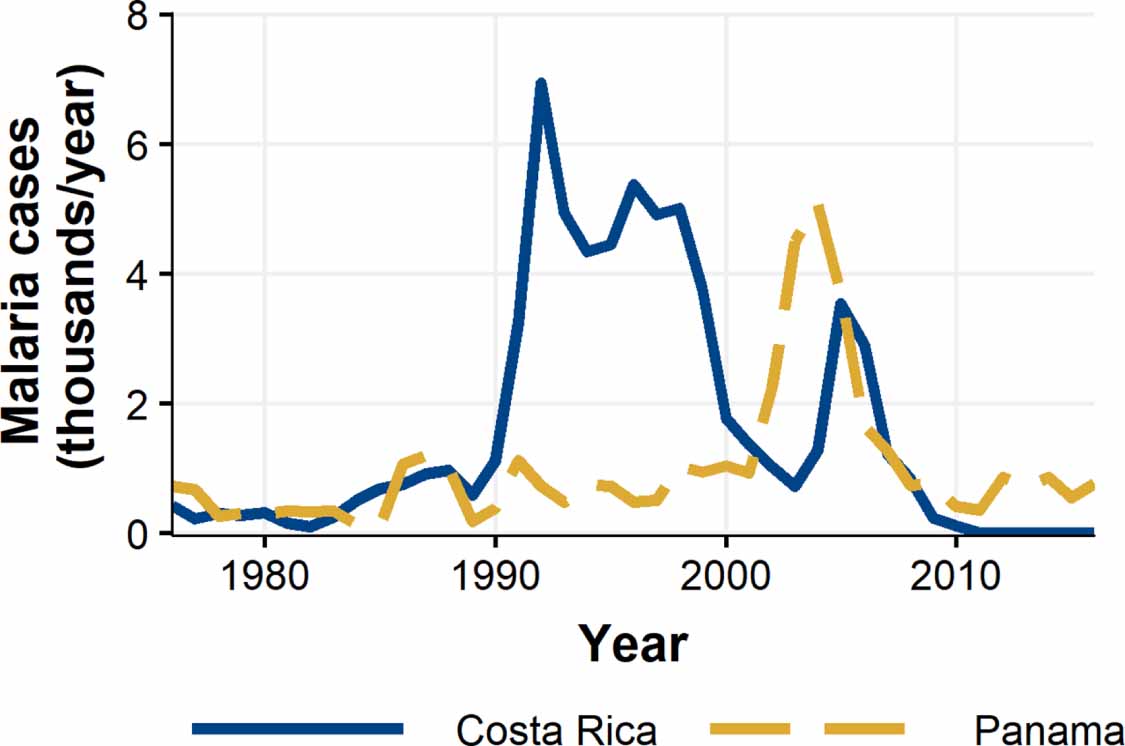
We take advantage of a natural experiment to provide what is to our knowledge the first causal empirical evidence of a negative human health impact associated with widespread amphibian loss, namely increased malaria incidence. Specifically, we focus on Central America where biologists have tracked an invasion wave of Bd that has decimated amphibians over the past few decades [7] 6 . This wave travelled from northwest to southeast across Costa Rica from the early 1980s to the mid-1990s and then continued eastward across Panama through the 2000s [7]. After this rolling collapse of amphibian populations, both countries experienced large increases in malaria cases. Figure 1 shows annual total malaria cases in Costa Rica and Panama for the time span of our analysis. While the ordering and timing of peaks in the two countries are consistent with a lagged impact of amphibian decline, this correlation does not establish a causal link on its own. To study this link more carefully we leverage local-level data as detailed below. To preview our main results, following the estimated date of Bd-driven amphibian decline in each 'county'—Costa Rican canton or Panamanian distrito—we find that malaria cases are significantly elevated for several years. For the six year peak of the estimated effect, the annual expected county-level increase in malaria ranges from 0.76 to 1.1 additional cases per 1000 population. This is a substantial increase given that cases country-wide per 1000 population peaked during the time frame of our study (see figure 1) at approximately 1.5 for Costa Rica and 1.1 for Panama.
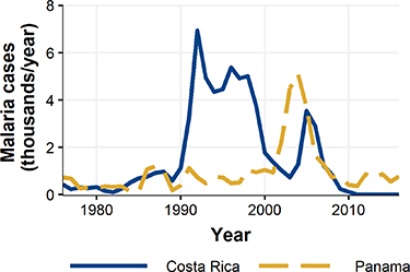
Figure 1. Annual total malaria cases from 1976 to 2016 for Costa Rica and Panama.
Download figure:
Standard image High-resolution imageThe global burden of malaria in 2018 included an estimated 228 million cases and 405 000 deaths, largely in sub-Saharan Africa and India [9]. Multiple overlapping social and environmental drivers have been linked with elevated malaria incidence. These include weather patterns, deforestation, human migration, and problems experienced by anti-malaria programs [10, 11]. Deforestation in particular has received increased attention in recent years and is hypothesized to operate through changes to the physical environment, malarial mosquito biology, and human exposure [12]. While most have found that deforestation is associated with increased malaria incidence [13], this result does not hold across all regions and study designs [14]. However, linkages between malarial dynamics and ecosystem disruption by invasive pests or pathogens has not been previously studied, aside from well-known linkages to invasive mosquito vectors.
Studying the real-world impacts of amphibian declines on malaria incidence is challenging. In a hypothetical idealized experiment, one would be able to (A) randomly distribute shocks to amphibian populations over a wide landscape, and (B) record detailed human malaria incidence as well as amphibian and mosquito densities over both space and time. For obvious ethical reasons, such an experiment cannot be conducted in the field. Our next best alternative for investigating the impact of amphibian declines on malaria—at scale and on the ground—is to identify a natural experiment, i.e. a natural shock to amphibian populations that can be cleanly characterized and does not impact other known socioeconomic drivers of malaria. While amphibian disease outbreaks provide one such opportunity, in much of the world their decades-long, region-wide effects are difficult to impossible to identify cleanly since they do not follow straightforward pathways over land. However, the Bd wave we study is ideal in this regard since it flowed from northwest to southeast through the isthmus of Central America. Progression through this narrow strip of land resulted in a relatively straightforward, unidirectional wave of shocks to amphibian populations. Furthermore, as we show below, the spatio-temporal pattern of the Bd wave is not systematically correlated with other potential drivers of malaria, including forest cover loss and precipitation patterns.
Because this Bd wave began in the early 1980s and lasted a few decades, consistent data coverage is a challenge. Detailed information is available for malarial incidence, human population, land cover and weather, which we combine with an ecological dataset of dates and locations of Bd-driven amphibian declines. Overall, the natural experiment provides exogenous variation in amphibian populations that allows us to uncover statistical evidence that Bd-driven decline in amphibians was associated with an increase in malaria. However, one key limitation is the absence of data on mosquito densities. This means we are unable here to take the additional step of providing empirical evidence that mosquitoes are the particular mechanism for the effect. Thus, we stress throughout this article that our new evidence pertains solely to the association between amphibian decline and malaria incidence.
Given this empirical limitation, it is crucial to elucidate existing evidence from the literature that such a link between amphibian and malaria dynamics is indeed plausible, e.g. as mediated by mosquitoes. There is much evidence to show that loss of amphibian species affects natural food webs with the potential to increase insect abundance, including mosquitoes capable of transmitting human diseases [15–22]. These species have been shown to influence mosquito populations through multiple channels, including predation, habitat selection (predator intimidation) and competition.
While adult caudate (salamander) and anuran (frog and toad) diets likely include adult mosquitoes and their larvae, existing studies have mainly focused on the impact of larval stage amphibians [19]. Lab studies confirm that some larval salamanders can consume high numbers of mosquito larvae, up to 400 per individual per day [16, 23]. Tadpoles from some anuran species have also been identified as strong consumers of mosquito larvae [19, 23]. For example, motivated by the role of mosquitoes like Aedes aegypti as a vector of diseases, Salinas et al [20] showed that tadpoles of a native frog species (Phyllodytes luteolus) preyed on mosquito larvae (from the family Culicidae) in field samples from Brazil. Amphibian-mosquito habitat selection impacts may be even greater. A large meta-analysis of amphibian, fish and invertebrate studies showed that the average impact of direct predation is exceeded by the impact of predator intimidation on prey demographics, through 'stimulating costly defensive strategies' [21]. Multiple field trial studies have found that mosquitoes shied away from ovipositing in sites with either tadpoles or larval salamanders [17, 24, 25]. A final pathway for amphibian-mosquito interaction at the larval stage stems from competition for limited resources in food networks [19]. Overall, Durant and Hopkins [16] point out that even if mosquitoes form a small share of amphibian diets, their sheer density 'could have a substantial impact on mosquito larvae abundance'. For example, Brodman et al [22] found that the presence of larval salamanders in wetlands coincided with a 98% drop in mosquito larvae density relative to those without.
Anopheles albimanus is the dominant malaria vector species from Mesoamerica through northern South America [26–28]. An. albimanus is a generalist species, with larval sites observed in both natural and developed areas with sunlit water [29]. These mosquitoes can develop across a wide range of breeding sites, varying in water type (e.g. swamps, ponds, marshes, rivers and irrigation channels) [29] and condition (e.g. 'salinity, turbidity and pollution') [30]. While adults are typically exophagic and exophilic—feeding and resting outdoors—their flying range exceeds 30 km and biting behavior is flexible, spanning from humans to animals and from outdoors to indoors [30, 31]. An. albimanus also shows wide tolerance across elevation (through 1900 m) though it is usually found below 500 m above sea level [31].
The set of amphibian species in Costa Rica and Panama is highly diverse, consisting of caecilians, salamanders and anurans. Excluding the fossorial caecilians (unlikely predators of dipteran insects) 182 species of salamanders and anurans have been recorded in Costa Rica [32] and 189 in Panama [33]. These amphibians are observed in diverse habitats and life zones, ranging from the coast to 3620 m above sea level, with 43%–52% of species registered at an altitude below 500 m [32, 33].
In our study region there is a gap in specific studies focused on amphibian-Anopheles albimanus interactions in particular as well as amphibian-mosquito interactions in general. The best available information is general, i.e. (a) Anopheles albimanus use water locations where larval and adult amphibians are also present and, (b) both Anopheles albimanus and amphibian species are found in a wide variety of natural, periurban and urban locations.
While multiple articles cited above discuss amphibian-mosquito interactions in the context of moderating disease risk to humans [16–18, 20] this link has been notoriously difficult to study. As Hocking and Babbitt [18] state in their review of amphibian contributions to ecosystem services, while the degree to which 'amphibian effects on mosquitoes translate to the spread of human diseases [including] malaria remains to be examined,' the 'major declines serve as natural experiments to understand the role of amphibians in ecosystems'.
In their 2021 review, de Vocht et al [34] note that natural experimental studies in public health 'can provide strong causal information in complex real-world situations, and can generate effect sizes close to the causal estimates from randomized controlled trials (RCTs)'. We leverage our particular natural experiment by using an event-study model to estimate the link between Bd-driven amphibian decline and malaria incidence at the canton level in Costa Rica and distrito level in Panama, hereafter referred to as 'county level'. This model exploits variation in outcomes for units (counties) that experienced the 'treatment' event (amphibian decline) at different times, which is a difference-in-difference (DID), event-study design [35]. Wing et al [35] detail methodological best practices and many peer-reviewed studies in this area, noting that the 'DID design is well established in public health research' and is 'often use(d) to study causal relationships in public health settings where RCTs are infeasible or unethical'. This DID approach is also standard in the econometric literature in cases where multiple units, such as states or counties, receive the same 'treatment' at different times [36–38]. We implement the method Wing et al [35] describe for time-varying treatment effects (p 460) in our model below, thus providing causal empirical estimates of the impact of Bd-driven amphibian decline on malaria incidence 7 .
Some research designs exploring similar questions seek to exhaustively include all potential covariates. However, in a DID event-study framework this is not the case. Instead, the task is to isolate the effect on the outcome of interest of a particular 'event'—here the county-level onset of systematic decline of amphibians due to spread of Bd. We take advantage of the staggered treatment of counties, i.e. differences in malaria outcomes over time between administrative units that have and have not been treated with Bd. This procedure allows us to pool information from the comparisons of treated and untreated counties, both before and after treatment. In a well-conceived event-study model, omitting other drivers (covariates) of the malaria outcome will not substantially impact the estimate of the effect of the event as long as these other drivers are not systematically correlated with the event (in our case, the wave of amphibian decline). In our key estimates below, we find a statistically significant relationship between Bd arrival at the county level and increases in malaria incidence. As long as the spatiotemporal spread of Bd-driven amphibian decline is uncorrelated with other potential drivers of malaria, their exclusion from the estimating model should not matter. Indeed, within our broader set of robustness checks, we show that adding/removing other known and possible malarial drivers has essentially no impact on our key estimates.
We highlight the scientific gap posed by the lack of historical mosquito density data to definitively pin down this vector's role in the pathway. However, important insights are still obtainable from the data that do exist in this natural experiment, i.e. the linkage between amphibian decline and malaria incidence as illustrated here. de Vocht et al [34] note that such natural experiments 'are appealing because they enable the evaluation of changes to a system that are difficult or impossible to manipulate experimentally (and) allow for retrospective evaluation when the opportunity for a trial has passed,' as is the case in our setting. Looking forward, our findings underscore the importance of adding collection of overlapping density data on both amphibians and disease vectors (mosquito and others) to the implementation of nascent surveillance systems, like the Australian Terrestrial Ecosystem Research Network or the US National Ecological Observatory Network [43], which is not currently planned to our knowledge. Establishing a baseline and tracking dynamic changes will be crucial for further deepening our understanding should the spread of another fungus—e.g. Batrachochytrium salamandrivorans, an emergent pathogen closely related to Bd—come to pass [4].
2. Results
To estimate the DID event-study model, we constructed a panel dataset spanning 41 years (annually from 1976–2016) and 136 counties in Costa Rica (81) and Panama (55), as detailed in the SM appendix. The outcome variable is malaria incidence (number of cases per 1000 population) from the parasites P. vivax and P. falciparum, with the vast majority of cases stemming from the former. The central driver of interest is the Bd-driven DoD of amphibians for each county. Bd spread is modeled across both countries since field observations of Bd impacts in our study region range from the lowlands [44–47] through high elevations [45, 46, 48]. To estimate county-level DoD values, we used all available field observations of the DoD at several sites across the two countries, specifically those directly labeled with years in figure 2. For a grid overlaying the region, we estimated a pixel-to-pixel Bd spread model fitted to these observed sites. The parameters selected to optimize the fit are the rates of spread at each of the DoD data points, which are extrapolated to all pixels—using ordinary Kriging—enabling the simulation of spread from initial arrival at the norther border of Costa Rica. Under this best-fit spread model, we set each county-level DoD to the earliest estimated DoD across all pixels in the county (when the edge of the jurisdiction is first reached). Figure 2 shows the estimated DoD for each county included in our preferred specification. See the SM appendix for further estimation detail. We excluded some counties, mainly in eastern Panama (indicated in figure 2) where precise DoD values were not available. The pattern shows a west-to-east wave spreading from the northwestern border of Costa Rica around 1980 to the Panama Canal region by 2010. In the SM appendix and later in our results we examine robustness to alternatives to both the spread model used and the summary DoD value used for the county.

Figure 2. Date of Bd-driven amphibian decline (DoD) in Costa Rica and Panama. Observed DoD points are directly labeled with years. Color shading indicates county-level earliest DoD, estimated using a spatial spread process model. Hashing indicates counties excluded in the preferred specification.
Download figure:
Standard image High-resolution image2.1. Effect of amphibian decline on malaria
Using the event-study regression model, we estimate the impact of Bd-driven amphibian decline on per capita incidence of malaria, while controlling for other potential covariates–see equation (1) in section 4. These estimates can be interpreted as causal as long as there are no omitted time-varying, county-level variables that both (A) impact malaria incidence, and (B) are correlated with the wave of Bd-driven amphibian decline from west to east in our time frame. We argue that it is extremely unlikely that there exists such a variable that would satisfy both conditions, especially the second. This assumption would be violated for instance if each county received medical funding in a way that was systematically correlated with the decline of amphibian populations in these counties. However, such omitted systematic correlation is very unlikely.
The key coefficients of interest (γk
) indicate the relationship between the number of malaria cases per thousand inhabitants and the number of years (k) since the DoD (date of amphibian population decline) in each county, conditional on the covariates. In figure 3 we plot the coefficients for each year k relative to the DoD along with 90% confidence intervals for the preferred regression model. For example, the coefficient for year k = 5 indicates the estimated effect on malaria cases once five years have passed since the DoD in the county. Similarly, the coefficient for year  estimates the effect several years before the DoD, which we expect to be indistinguishable from zero if the model is well specified. More broadly, a crucial validity test of our event study framework is to confirm the absence of a pre-trend, i.e. a directional trend in the effect on malaria cases of the year relative to amphibian decline before treatment at year 0. Simply put, we would not expect to see systematic movement in malaria incidence in years before amphibian decline begins. We confirmed lack of such a pre-trend: none of the coefficients for k < 0 are significantly different from zero
8
.
estimates the effect several years before the DoD, which we expect to be indistinguishable from zero if the model is well specified. More broadly, a crucial validity test of our event study framework is to confirm the absence of a pre-trend, i.e. a directional trend in the effect on malaria cases of the year relative to amphibian decline before treatment at year 0. Simply put, we would not expect to see systematic movement in malaria incidence in years before amphibian decline begins. We confirmed lack of such a pre-trend: none of the coefficients for k < 0 are significantly different from zero
8
.

Figure 3. Estimated effect on malaria cases per 1000 population (vertical axis) of year k (horizontal axis) relative to Bd-driven date of amphibian decline (DoD). Confidence intervals are given by shading (95%) and dashed lines (90%).
Download figure:
Standard image High-resolution image
Overall, we estimated a significant increase in malaria cases due to the onset of amphibian decline, an effect that starts gradually, plateaus after three years, and starts to attenuate after eight years. The first year of amphibian decline (k = 0) reflects partial treatment for most counties since Bd-saturation of a county takes a median of 1.1 years and spread may arrive anytime in a calendar year. Starting in year k = 1, amphibian decline is associated with a statistically significant increase in malaria cases. We estimate that this average effect reaches a relative plateau by year k = 3 and stays relatively constant for six years. For one year in this range (k = 6) the effect is not significantly different from zero. This is not due to a decline in the coefficient but rather to an increase in the standard error due to an increase in residuals, i.e. additional noise. Starting in year k = 9 the average effect begins to attenuate and is no longer significantly different from zero.
For perspective on the relative magnitude of this Bd-driven effect, peak cases per 1000 population reached approximately 1.1 for Panama (2002–2007) and 1.5 for Costa Rica (1991–2001). For the six years our estimated effect of amphibian decline is at its highest, the annual expected increase in malaria ranges from 0.76 to 1.1 additional cases per 1000 population. This represents a substantial share of cases overall.
2.2. Robustness checks
In table 1 we present the full set of regression estimates for the preferred specification (discussed above) in column 1, alongside estimates for three alternative specifications (columns 2–4) to check robustness (discussed further below). In the table, regression coefficients are presented with standard errors in parentheses, which are clustered at the county level. We clustered due to the sampling design (we are inferring something about the larger population based on data sampled at the county level) and our quasi-experimental design ('treatment' occurs at the county level). Overall, we found that our key qualitative results discussed above hold across an array of robustness checks.
Table 1. Estimates for the regression model specified in equation (1) for the preferred specification (column 1) and alternatives for robustness checks. Standard errors (clustered at the county level) are presented in parentheses.
| Dependent variable: malaria cases per 1000 population | ||||
|---|---|---|---|---|
| Preferred specification | All observations | Average date of decline | Weighted regression | |
| (1) | (2) | (3) | (4) | |
| Tree cover | −2.476 (1.162) (1.162) | −2.819 (1.175) (1.175) | −2.490 (1.157) (1.157) | −1.934 (0.858) (0.858) |
| Bare ground | −1.930 (1.438) | −2.343 (1.429) | −1.844 (1.368) | −1.317 (0.754) (0.754) |
| Precipitation | 0.003 (0.002) | 0.003 (0.002) | 0.003 (0.002) | 0.001 (0.001) |
| Av. Temp. | −2.289 (0.609) (0.609) | −3.003 (0.636) (0.636) | −1.885 (0.602) (0.602) | −1.619 (0.493) (0.493) |

| −0.418 (0.152) (0.152) | −0.381 (0.167) (0.167) | −0.535 (0.191) (0.191) | −0.307 (0.101) (0.101) |

| −0.129 (0.165) | −0.081 (0.204) | −0.238 (0.184) | −0.129 (0.100) |

| −0.175 (0.158) | −0.194 (0.182) | −0.259 (0.154) (0.154) | −0.115 (0.087) |

| −0.190 (0.139) | −0.325 (0.170) (0.170) | −0.247 (0.134) (0.134) | −0.131 (0.087) |

| −0.128 (0.081) | −0.200 (0.119) (0.119) | −0.212 (0.086) (0.086) | −0.052 (0.062) |

| 0.087 (0.083) | 0.085 (0.084) | 0.201 (0.096) (0.096) | 0.038 (0.049) |

| 0.203 (0.129) | 0.139 (0.138) | 0.433 (0.213) (0.213) | 0.105 (0.075) |

| 0.376 (0.168) (0.168) | 0.278 (0.172) | 0.695 (0.271) (0.271) | 0.313 (0.129) (0.129) |

| 0.786 (0.272) (0.272) | 0.773 (0.265) (0.265) | 0.692 (0.288) (0.288) | 0.745 (0.317) (0.317) |

| 0.851 (0.304) (0.304) | 0.896 (0.299) (0.299) | 0.649 (0.362) (0.362) | 0.844 (0.383) (0.383) |

| 0.755 (0.326) (0.326) | 0.888 (0.327) (0.327) | 1.050 (0.693) | 0.656 (0.270) (0.270) |

| 0.974 (0.597) | 1.016 (0.582) (0.582) | 0.947 (0.528) (0.528) | 0.665 (0.397) (0.397) |

| 1.080 (0.472) (0.472) | 1.194 (0.469) (0.469) | 0.646 (0.450) | 0.877 (0.375) (0.375) |

| 1.008 (0.492) (0.492) | 1.176 (0.488) (0.488) | 0.371 (0.353) | 0.740 (0.351) (0.351) |

| 0.641 (0.364) (0.364) | 1.096 (0.469) (0.469) | 0.279 (0.347) | 0.484 (0.264) (0.264) |

| 0.437 (0.317) | 0.791 (0.374) (0.374) | 0.218 (0.329) | 0.324 (0.239) |

| 0.876 (0.454) (0.454) | 0.952 (0.449) (0.449) | 0.682 (0.478) | 0.667 (0.328) (0.328) |
| Mean outcome | 0.45 | 0.61 | 0.45 | 0.45 |
| No. clusters | 136 | 144 | 136 | 136 |
| Observations | 5576 | 5904 | 5576 | 5576 |
| Adjusted R2 | 0.302 | 0.313 | 0.302 | 0.311 |
*p < 0.1; **p < 0.05; ***p < 0.01. Note: In the preferred specification: observations are unweighted and counties with an imprecise date of decline (DoD) are excluded; and county DoD is from the pixel-to-pixel spread model and is set to the earliest DoD across pixels in the county. Weighted regression uses county-level population weights.
In the table, our independent variables (rows) start with two ground cover measures and two weather measures. Next are the key coefficients of interest,  , representing the estimated effect of relative years before a county's DoD (k < 0) and after (
 ). These coefficients for our preferred specification for
  are plotted in figure 2 and discussed above. We excluded
  so that the rest of these coefficients are interpreted as effects relative to this year just before a county's DoD. For our first alternative specification in column (2) we augmented the data set with regions of Panama excluded in our preferred specification due to data limitations as described in the SM appendix. (Excluded regions included eastern Panama and the re-aggregated district 'Bocas del Toro'.) In column (3) we considered an alternative rule for converting the raster of DoD levels at the pixel-level to the county-level: instead of the using the minimum date reflecting initial arrival to the county border, we considered the average DoD for the county. In column (4) we conducted weighted least squares regression where the weights were given by county-level population. This heightened emphasis on observations from high-population counties is motivated by the conjecture that malaria incidence measures from such counties are less subject to measurement error (ME) given the larger number of 'samples' available. (However, further below we note that denser counties in our sample typically have lower base levels of malaria incidence and explore how this affects our estimates by dropping such units.)
For our key coefficients of interest, under our preferred specification none of the pre-DoD coefficients ( for
for ![$k \in [\kern-1.5pt[-5,-2]\kern-1.5pt]$](https://content.cld.iop.org/journals/1748-9326/17/10/104012/revision1/erlac8e1dieqn75.gif) ) are significantly different from zero, i.e. we fail to find a significant pre-trend in malaria in the five years leading up to the DoD. In event study frameworks like the one used here, such a lack of a pre-trend is one critical check for model validity. In subsequent relative years after Bd-driven amphibian decline, the coefficients are positive, significantly so for
) are significantly different from zero, i.e. we fail to find a significant pre-trend in malaria in the five years leading up to the DoD. In event study frameworks like the one used here, such a lack of a pre-trend is one critical check for model validity. In subsequent relative years after Bd-driven amphibian decline, the coefficients are positive, significantly so for  , with the exception of one year (k = 6). Lack of significance in this year appears to stem from an uptick in noise—the coefficient is within the range of surrounding years while the standard error is elevated.
We found that the same general pattern holds across all specifications: we fail to find a pre-trend before the DoD and then find a block of significant positive effects on malaria subsequent to the DoD. This pattern shifts earlier in relative years under specification (3) as we would expect. In this specification k = 0 does not indicate the beginning of treatment but rather a time when approximately half of the county has already been treated. In this case the omitted year  (for which the effect is assumed to be zero) includes partially treated counties, skewing the baseline and leading to a likely spurious significant negative coefficient for
  . This justifies focus on our preferred specification in which all treatment begins at k = 0, aiding consistent interpretation of the coefficients.
As additional robustness checks, we examined the sensitivity of our results to two alternative methods for estimating the gridded DoD levels (see the SM appendix for detailed methods). In the first alternative, we extend our baseline spread model to allow for elevation-dependent spread rates. This is motivated by the fact that laboratory studies show Bd thrives in a temperature band found at medium and higher altitudes in our study region [49, 50], which is also where we observe more contiguous natural habitat. In the second alternative we replace our baseline spread model with a thin-plate spline (TPS) method for directly estimating DoD from the data via interpolation over space. The TPS approach is appealing in its single-step simplicity, though it ignores the implications for spread of Central America's irregular coastline. We find that results from both alternatives are broadly consistent with our preferred specification, with significant increases in malaria by year 2–3 after the DoD (see figures S3 and S4). Even so, prospects for DoD ME remain in our preferred specification. We discuss the implications for such DoD ME in detail in the SM appendix. The main implications are stronger prospects for a significant pre-trend before the DoD and dampened initial post-DoD coefficients. While we cannot entirely rule out these effects, we do not find a significant pre-trend and our post-DoD coefficients remain significant. Still, in the detailed appendix discussion, we outline conditions under which the arc of the post-DoD coefficient curve could be affected, motivating caution against sharp emphasis of exact estimates.
2.3. Additional drivers of malaria
We also found that decreasing tree cover is associated with a statistically significant increase in malaria cases under all specifications (see first row of table 1) in keeping with the majority of findings of previous studies. A one standard deviation decrease in tree cover (0.05) is associated with an increase of 0.12 in the number of cases of malaria per 1000 inhabitants. This is about one-ninth the magnitude of the estimated amphibian decline impact at its peak. Bare ground also has a negative effect on cases, though this effect is not consistently significant. Non-tree vegetation, the third land cover type, was excluded from the regression because all three types sum to one for each county; the excluded type is perfectly multicollinear with the sum of the two included measures.
For weather variables, the results were consistent across specifications: higher average temperature was significantly associated with fewer cases, while increasing precipitation was associated with more cases, though not significantly so. In the SM appendix (table S3) we show regression results for alternative specifications of temperature effects (nonlinear effect of average temperature; minimum and maximum temperature; the difference between minimum and maximum temperature). We find that no alternative temperature variable in any of these configurations is significant.
While in some research designs we seek a comprehensive model of the outcome, in a DID event study framework we do not necessarily seek to include every plausible covariate. Instead, the focus is on isolating the effect on the outcome of interest of a particular 'event'—here the county-level onset of systematic decline of amphibians due to spread of Bd. Omission of other drivers of the malaria outcome (covariates) should not impact the estimate of the effect of the event as long as these other drivers are not systematically correlated with the event (wave of amphibian decline). We illustrate this feature of our model by (A) removing our existing covariates (weather and land cover), and separately (B) adding an additional covariate (population), and showing that both have a negligible effect on our key estimates (see table S4 in the SM appendix). This is an expected feature of an effective natural experiment: because other potential drivers of malaria are uncorrelated with our event of interest, their inclusion/exclusion has essentially no impact on the estimate of amphibian decline on malaria incidence. In this vein, loss of tree cover itself is likely to negatively effect amphibian populations. However, this is unlikely to affect our qualitative results since this given that inclusion or exclusion of land cover variables has a negligible effect on our key estimates (as one would expect when forest cover dynamics are not systematically correlated with the Bd-driven wave of amphibian decline).
Our event-study estimates in table 1 reflect the average county-level effect. A natural approach to examine whether impacts vary by county in a systematic way is to interact the event study coefficients (γk ) with quantiles of county variation in a given measurement (e.g. as in [51]). However, since the number of observations in our sample is insufficient for this approach we instead simply consider the impact on the event study coefficients of dropping from our sample the 20 or 40 counties (out of 136 overall) with the most extreme values for a given measure. Since results in table 1, columns (1) and (4), show that adding county population weights slightly decreases estimates, we assess sensitivity to dropping counties with the highest population density (2010 population per square kilometer). In results shown in SM appendix table S5, we find that the magnitude of the post-DoD effect estimates (and their significance level) increases noticeably after dropping 20 counties, and even more so when dropping 40. One possible explanation is that other factors correlated with population density, like elevation or temperature could be contributing. However, when dropping counties with the lowest elevation or highest temperature we find that post-DoD effect estimates are either very slightly higher for a subset of coefficients (elevation) or essentially unchanged (temperature). Another explanation is that malaria risk in counties with denser population is simply lower in general. The data support this explanation–denser counties in our sample exhibits substantially lower level of malaria cases overall. However, urban areas typically have less diversity and abundance of amphibians relative to periurban and natural areas [32]. Lack of amphibian abundance data over space and time at the country scale makes it difficult to separate this effect from other factors associated with population density.
3. Discussion
Overall we provide novel causal empirical evidence that pathogen-driven amphibian decline can play a significant role in increasing incidence of insect-borne disease. Our results also contribute to a nascent but growing literature identifying indirect and previously unknown impacts of invasive species on human health [52–54]. If scientists and decision makers fail to reckon with the ramifications of such past events, they also risk failing to fully motivate protection against new calamities, like international spread of an emergent and closely related pathogen Batrachochytrium salamandrivorans through incompletely regulated live species trade [4].
While results were robust to several alternative specifications, we were unable to examine whether Bd-driven amphibian decline was associated with changes in other diseases. Other insect-borne diseases, such as dengue and leishmaniasis, have their own ecological dynamics, distinct from malaria. This is particularly true for leishmaniasis which is caused by parasites carried by phlebotomine sand fly species that (to our knowledge) are not known to be preyed on by amphibians but rather may use amphibians as a blood source [55, 56]. Identifying a significant change in incidence of either disease associated with Bd-driven amphibian decline would have provided additional support for the importance of ecological feedbacks. Conversely, showing that an association failed to hold for non-insect-borne illnesses like influenza would increase support for the argument that the effect we identify is specific to insect-borne diseases and not a general disease effect. We attempted to obtain these disease data sets from the national ministries of health in both countries but they were not available for our period of study at the county-level needed.
From the data we were able to obtain from the Panamanian Ministry of Health (shown in SM appendix figure S6) we found that, similar to the spike observed in malaria cases for 2002–2007 shown in figure 1, the national-level time series for both dengue and leishmaniasis show elevated cases in this time range. Relative to a baseline from the preceding ten years, average annual leishmaniasis cases were 22% higher for 2002–2007. For dengue the increase relative to the previous eight years (all available) was 36%. When we extended the window of potential impact to 2002–2011, average annual cases increased relative to baselines by 23% and 61%, respectively.
Our results suggest that the level of increase in malaria incidence subsequent to Bd-driven amphibian decline was substantial relative to country-wide annual incidence during the time frame of our study in Costa Rica and Panama, which peaked at 1.1 and 1.5 per 1000 population, respectively. While this is a significant health burden for these two countries, we note that this level of incidence is much lower than peaks observed in the last two decades elsewhere in the region (e.g. 200–300 for Ecuador and Suriname in the early 2000s) and especially relative to equatorial Africa (with 18 countries above 400 in the early 2000s and 11 still in the 300–400 range in 2020) [57].
While the focal shocks of interest here are initially to biological and ecological factors, we would expect behavioral responses to play a role, especially in the longer run. For example, one key question emerging from our results is why the estimated effect (of Bd-driven amphibian loss) attenuates, here after approximately eight years. One plausible explanation is an increased malaria prevention program response to an observed uptick in malaria cases, e.g. increased investment in control measures like insecticide application. In the SM appendix we discuss indicators of national malaria prevention actions (total funding and number of houses sprayed for mosquitoes) for our period of study for both countries [58]. Total funding dynamics in both countries show increased (though sometimes uneven) investment in malaria prevention following national outbreaks, which would plausibly serve to suppress cases over time. While the evidence is suggestive we were not able to include these time series in our regression model since they are not available at the county level.
Behavioral responses could also complicate the process on a shorter time scale, e.g. if noticeable effects of Bd-driven decline in one county (e.g. increase in mosquitoes and/or malaria cases) were to drive an increase in mosquito and/or malaria mitigation measures in counties not yet experiencing the effects. If true, this would bias our estimates of the effect of Bd-arrival on malaria incidence, specifically dampening them towards zero. While possible, we view this as unlikely given the time delay to put such mitigation measures into place and the propensity to focus such measures in places where cases have already spiked.
The case for interpreting our estimated effects (of Bd-driven amphibian decline on malaria incidence) as causal rests on the assumption that there are no omitted time-varying, county-level variables that both (A) impact malaria incidence, and (B) are correlated with the wave of Bd-driven amphibian decline from west to east in our time frame. To support this argument, we have shown that our qualitative results are robust to inclusion and exclusion of other covariates known to impact malaria incidence. Even so, for such an observational study, caution is warranted since it is not possible to unequivocally rule out the existence of some social or ecological confounding factor that may have been correlated with the Bd-driven wave. As such, our results are arguably best-viewed as a first but not final piece of evidence on the topic, which would benefit from the application of additional data collection and alternative study designs, e.g. to test the individual links in the overall chain of effects we propose here.
4. Methods
We specified the event-study regression model as
where Mct
is malaria cases per thousand inhabitants in county c and year t. The Bd-driven date of decline for county c is given by  , where the unit is year. Also, at time t the number of years relative to this event is given by
  . For example, if county c is 'treated' by the arrival of Bd-driven amphibian decline at the start of 1990, then at t = 1992, the year relative to the event is
  ; county c has completed two years of treatment and is entering its third. Our main regressor of interest is τck
, which is a dummy variable equal to one if county c is k years away from the initial treatment event:
; county c has completed two years of treatment and is entering its third. Our main regressor of interest is τck
, which is a dummy variable equal to one if county c is k years away from the initial treatment event:  . We focus on the five relative years before the event and ten years following:
  . We also included a single dummy for all relative years before this, denoted by
  and another for all relative years after,
  . Allowing the coefficient γk
to vary for each relative year (Kct
) in this way facilitates flexible and dynamic treatment effects. Because we imposed
. Allowing the coefficient γk
to vary for each relative year (Kct
) in this way facilitates flexible and dynamic treatment effects. Because we imposed  to serve as the baseline, the remaining coefficients γk
are interpreted as effects relative to the year
to serve as the baseline, the remaining coefficients γk
are interpreted as effects relative to the year  , the year just before the DoD.
A vector of time-varying, county-level control variables is given by  . These include two annual weather measures: total precipitation and average temperature. We also consider annual land cover variables (share of tree cover, non-tree cover and bare ground) to account for the role of deforestation.
The regression model in equation (1) also includes county fixed-effects (individual county dummies λc
) to control for differences between spatial units that are constant over time (e.g. elevation) as well as year fixed effects (individual year dummies λt
) to control for any shocks that affect malaria incidence in all counties in a given year. Rounding out the model,  ct
is a county-level error term.
ct
is a county-level error term.
Acknowledgments
We thank L Fonseca for research assistance, R Hijmans for spatial modeling advice, and the following individuals for assistance obtaining malaria data: M Piaggio (Environment for Development); T and R Castro (Costa Rica Ministry of Health); and D Batista, E Benavides, M Lasso and L García (Panama Ministry of Health). We also thank D Rodríguez and L Moreno (Panama Ministry of Health) for providing the leishmaniasis and dengue data. For their helpful comments, we thank participants of the University of California Davis NatuRE Policy Lab, University of Colorado Environmental and Resource Economics Workshop, Association of Environmental and Resource Economists conference, and two anonymous reviewers.
Data availability statement
All data and code for reproducing results is available at GitHub https://github.com/JoakimWeill/Amphibian_collapses_ERL.
Funding
Research was funded by NSF DEB-1414374 and the University of California Davis' John Muir Institute of the Environment; R I was supported by the Sistema Nacional de Investigación (SENACYT), Panama Amphibian Rescue and Conservation Project, and Minera Panamá; K R L was supported by NSF DEB-0717741 and DEB-0645875.
Author contributions
Conceptualization (K R L, M R S and J A W), Data curation (all), Methodology and Formal Analysis (M R S and J A W), Funding acquisition (M R S), Investigation (all), Project administration (M R S), Visualization (A G, M R S and J A W), Writing—original draft (M R S and J A W), Writing—review and editing (all).
Conflict of interest
The authors declare that they have no competing interests.
Footnotes
- 6
At minimum, Bd has significantly impacted dozens of amphibian species in our study region, with affects ranging from significant abundance decline to extirpation. However it is difficult to say precisely how many species have been affected since this relies on comprehensive surveying both before and after the Bd wave and this information is limited to a small number of sites. For the best studied site in the region (north of El Copé in Panama) after the arrival of Bd 30 amphibian species were no longer found and deemed extirpated (41% of the community previously present), 9 species showed critical population declines (85%–90% drop in abundance) and 9 more showed significant abundance declines (up to 55%) [8].
- 7
A recent literature highlights that interpreting event-study estimates as dynamic average treatment effects requires the underlying treatment effects to be homogeneous between treatment cohorts [39–42], i.e. between counties experiencing an amphibian date of decline (DoD) in a given year. It is not feasible to directly test this assumption, however, we show through a Bacon-Goodman decomposition [40] in SM appendix figure S5 that any potential bias introduced by heterogeneous treatment effects is unlikely to substantially affect our estimates.
- 8
In the SM appendix we provide a balance table S2 reporting the mean and spread at the county level for key variables pre and post DoD, or 'treatment'. The table shows a substantial increase (post treatment) in average malaria per thousand inhabitants, while the climate and land cover control averages are relatively stable.
Supplementary data (3.3 MB PDF)