the Creative Commons Attribution 4.0 License.

the Creative Commons Attribution 4.0 License.
A probabilistic framework for quantifying the role of anthropogenic climate change in marine-terminating glacier retreats
- 1Institute for Geophysics, University of Texas at Austin, Austin, Texas 78758, USA
- 2School of Earth and Atmospheric Sciences, Georgia Institute of Technology, Atlanta, Georgia 30318, USA
- 1Institute for Geophysics, University of Texas at Austin, Austin, Texas 78758, USA
- 2School of Earth and Atmospheric Sciences, Georgia Institute of Technology, Atlanta, Georgia 30318, USA
Correspondence: John Erich Christian (jchristian41@gatech.edu)
Hide author detailsCorrespondence: John Erich Christian (jchristian41@gatech.edu)
Many marine-terminating outlet glaciers have retreated rapidly in recent decades, but these changes have not been formally attributed to anthropogenic climate change. A key challenge for such an attribution assessment is that if glacier termini are sufficiently perturbed from bathymetric highs, ice-dynamic feedbacks can cause rapid retreat even without further climate forcing. In the presence of internal climate variability, attribution thus depends on understanding whether (or how frequently) these rapid retreats could be triggered by climatic noise alone. Our simulations with idealized glaciers show that in a noisy climate, rapid retreat is a stochastic phenomenon. We therefore propose a probabilistic approach to attribution and present a framework for analysis that uses ensembles of many simulations with independent realizations of random climate variability. Synthetic experiments show that century-scale climate trends substantially increase the likelihood of rapid glacier retreat. This effect depends on the timescales over which ice dynamics integrate forcing. For a population of synthetic glaciers with different topographies, we find that external trends increase the number of large retreats triggered within the population, offering a metric for regional attribution. Our analyses suggest that formal attribution studies are tractable and should be further pursued to clarify the human role in recent ice-sheet change. We emphasize that early-industrial-era constraints on glacier and climate state are likely to be crucial for such studies.
- Article
(5232 KB) -
Supplement
(2384 KB) - BibTeX
- EndNote


Many marine-terminating glaciers in Greenland and Antarctica have retreated in recent decades, causing increased discharge to the ocean and accelerating sea-level rise (e.g., Meredith et al., 2019; Mouginot et al., 2019; Rignot et al., 2019). In Greenland, marine-terminating glacier retreat has been widespread across the ice sheet, although heterogeneous within regions (Howat et al., 2008; Moon and Joughin, 2008; Murray et al., 2015; King et al., 2018; Catania et al., 2018). In Antarctica, grounding line retreat and dynamic thinning is underway in the Amundsen Sea Embayment (ASE; e.g., Rignot et al., 2014; Joughin et al., 2014), and widespread retreat of glacier termini has also been documented on the Antarctic Peninsula (Cook et al., 2014) and parts of East Antarctica (Miles et al., 2013).
In both Greenland and Antarctica, the retreat of grounded ice has been linked to ocean forcing (Holland et al., 2008; Straneo et al., 2013; Jenkins et al., 2016; Wood et al., 2021), which in many cases is also linked to atmospheric changes. For example, wind anomalies in the Amundsen Sea are thought to drive warm Circumpolar Deep Water towards ASE glaciers (e.g., Thoma et al., 2008), while in Greenland, surface meltwater from atmospheric warming is discharged subglacially at glacier termini and affects heat exchange between the ice and fjord waters in buoyant plumes (e.g., Straneo et al., 2011; Fried et al., 2015). In many cases, these local atmospheric and ocean anomalies can be traced to large-scale modes of internal climate variability. Tropical Pacific variability has been tied to submarine melt for ASE glaciers (Steig et al., 2012; Dutrieux et al., 2014; Holland et al., 2019), and canonical modes of North Atlantic Ocean and atmospheric variability have been concurrent with glacier retreat in Greenland, especially in the southern and central sectors of the ice sheet (e.g., Straneo et al., 2013; Khazendar et al., 2019). Though observations of glacier change are overwhelmingly concentrated in the last few decades, historical records and proxy evidence suggest links between these climate modes and glacier retreat earlier in the 20th century as well (e.g., Andresen et al., 2012; Bjørk et al., 2012; Andresen et al., 2014; Smith et al., 2017).
The sensitivity of marine-terminating glaciers to internal climate variability raises the question as to whether recently observed retreats are caused by natural variability or anthropogenic climate change. Arctic and Antarctic land-surface warming has been formally attributed to anthropogenic forcing (Gillett et al., 2008), and recent studies have identified anthropogenic trends in additional climate variables relevant to glacier forcing, such as the winds that modulate ocean circulation near western Antarctic glaciers (Holland et al., 2019; O'Connor et al., 2021). However, attribution of observed glacier retreats must incorporate the complex dynamics that link local climate to glacier response. Despite advances in understanding marine-terminating glacier dynamics and ice–ocean interactions in recent decades (e.g., Jenkins et al., 2016; Catania et al., 2020), observed retreats and the associated dynamic mass loss have yet to be attributed to anthropogenic forcing, as detailed in the IPCC's (Intergovernmental Panel on Climate Change) Special Report on the Oceans and Cryosphere in a Changing Climate (SROCC; Meredith et al., 2019) and most recent assessment report (AR6; IPCC, 2021).
Why have marine-terminating glacier changes not yet been formally attributed? Strong variability in high-latitude climate, multiple forcing processes, and limited observations are among the challenges reviewed in the SROCC and AR6. The dynamics of marine-terminating glacier flow and the potential for internal glacier instabilities pose additional challenges but have not yet been addressed in formal attribution analyses. In this study we propose a way forward, developing a probabilistic attribution framework that accounts for marine-terminating glacier dynamics in the context of natural climate variability. Before presenting our methods and results, we briefly review the key elements of previous climate attribution analyses and outline specific challenges that we will consider for marine-terminating glacier retreats.
Attributing changes in any part of the Earth system to anthropogenic forcing is typically accomplished by comparing model simulations of that system with anthropogenic forcings included to simulations in which anthropogenic forcings are omitted. For example, climate model simulations including all major natural (e.g., volcanic and solar) and anthropogenic forcings (e.g., greenhouse gases and aerosols) are compared against counterfactual simulations with only the natural forcings (e.g., IPCC, 2021). Only the simulations including all known sources of forcing on the climate system match observed warming trends, giving high confidence that the global-mean warming over the industrial era is attributable to human influence rather than natural forcings or internal variability. Another category of attribution studies focuses on extreme events, such as individual heat waves, floods, or storms (see, e.g., Stott et al., 2016, for a review). Because extreme events would still occur due to internal variability in a natural climate, these studies focus on how anthropogenic forcing changes the likelihood of a given extreme. Although this framing is different from that of trend attribution, these studies still rely on comparing simulations with and without anthropogenic forcing. For example, Stott et al. (2004) examined temperature extremes in climate model output and concluded that European heat waves as severe as that of 2003 had become at least twice as likely due to anthropogenic forcing. Many studies on subsequent events have followed, and methods for event attribution have become increasingly standardized (Philip et al., 2020).
Attribution studies within glaciology have thus far focused on mountain glacier losses over the industrial era (Marzeion et al., 2014; Roe et al., 2017, 2021). These studies require models that accurately capture how glacier dynamics integrate both long-term trends and short-term climate variability and that have shown that the loss of mountain glaciers over the industrial era is clearly attributable to anthropogenic forcing, both for the metrics of terminus retreat (Roe et al., 2017) and mass balance (Roe et al., 2021). Indeed, the kilometer-scale retreats of mountain glaciers are some of the most statistically robust indicators of anthropogenic climate change observed in the Earth system (Roe et al., 2017).
In all of these examples, attribution relies crucially on capturing the full scope of natural variability within a system. For marine-terminating glaciers, observations (discussed above), as well as theory and models (Robel et al., 2018; Christian et al., 2020), indicate that glacier termini fluctuate in response to stochastic climate variability. However, the largest observed retreats are overwhelmingly associated with retrograde bed slopes (i.e., deepening inland), both for marine-terminating glaciers in fjords in Greenland (Catania et al., 2018; Wood et al., 2018) and for large outlet systems in West Antarctica, such as Pine Island and Thwaites glaciers (Rignot et al., 2014; Joughin et al., 2014). This implicates the marine-ice-sheet instability (e.g., Weertman, 1974; Schoof, 2007), in which termini on retrograde beds may undergo runaway retreat if sufficiently perturbed due to a positive feedback between ice flux and thickness at the terminus. Retreats continue until the inland topography becomes sufficiently shallow (or laterally constricted), or they may lead to complete glacier retreat.
The cases where instabilities contribute to observed glacier-terminus retreats present a unique challenge for attribution studies because they raise the possibility that natural variability could trigger a retreat of the same magnitude as one driven by anthropogenic forcing. In other words, large marine-terminating glacier retreats are not necessarily indicators of a significant climate change. Just as extreme events require a different attribution framework compared to other climate phenomena, retreats of marine-terminating glaciers may also require a unique framework when dynamic instabilities are possible. Our guiding question in this study is thus, “what is the likelihood that natural variability alone drives rapid glacier-terminus retreat, and how does an anthropogenic trend in forcing change this likelihood?” To address this question, we introduce an ensemble-based attribution framework (Sect. 2.3) as a tool for assessing the retreat of single glaciers and groups of glaciers.
We emphasize that this study is not itself a formal attribution assessment for a particular glacier or region. Rather, we identify key physical principles that affect the likelihood of rapid marine-terminating glacier retreats in a noisy climate and show how model ensembles can be used to clarify the effects of anthropogenic forcing. It is worth noting here that our model simulations do not include floating ice shelves, which can alter the thresholds for dynamic instability via lateral buttressing (e.g., Gudmundsson et al., 2012). We focus instead on cases where stability is a function of bed topography, which simplifies our analysis of glacier variability near instabilities. Accordingly, we orient model parameters and the discussion of results around marine-terminating glaciers in Greenland, where floating ice plays a lesser role than in Antarctica. However, inasmuch as strongly buttressed glaciers and ice streams are still subject to climate variability and may be prone to instabilities, many of the fundamental points for attribution could be adapted for such settings (albeit with additional ice-shelf dynamics to capture). Our main goal is to put forward a probabilistic framework that can be used as a methodological guide for future attribution studies.
We first introduce the model and ensemble methods (Sect. 2). Second, we explore the null hypothesis of noise-triggered glacier retreat and analyze controls on the likelihood of such retreat (Sect. 3). Third, we assess the effects of anthropogenic forcing and present a synthetic attribution experiment (Sect. 4). Our final set of results shows how to frame attribution for a population of glaciers (Sect. 5). We close with a discussion of our findings, key uncertainties, and recommendations for how the community could proceed with formal attribution studies.
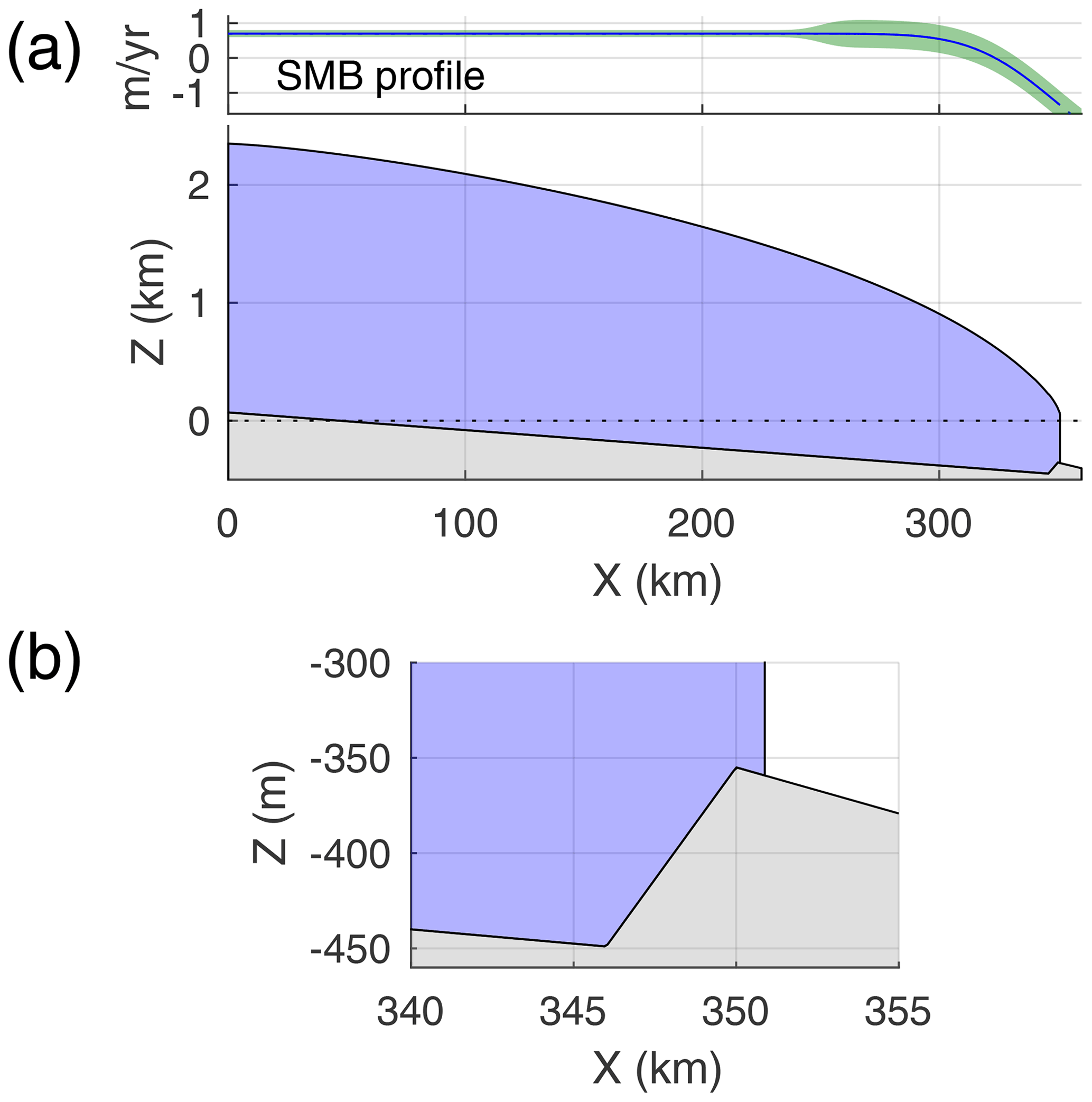
Figure 1(a) An idealized marine-terminating glacier, whose steady-state terminus position is approximately 1 km from a bed peak. SMB profile is shown on top; shading shows the magnitude of variability (1σ). (b) Close-up of the bed peak.
2.1 Glacier model and idealized geometry
We use a 1-D model of marine-terminating glacier dynamics that assumes flow is dominated by longitudinal stretching and Weertman-style sliding (see Supplement for equations). Ice velocities are calculated using the shallow shelf/stream approximation (SSA), ice thickness is calculated through mass conservation, and the terminus position is calculated using an implicit flotation condition. Following the numerical approach laid out in Schoof (2007), the governing equations are solved on a grid stretched to the glacier extent at each time step. That is, if the glacier advances or retreats, the grid nodes shift with respect to a fixed spatial coordinate. The model does not simulate any floating ice, so the last grid point always represents the grounding line (i.e., a terminus at flotation). The grid spacing is several kilometers through most of the interior but is significantly refined (∼100 m) near the grounding line. Ice flux across the grounding line is not parameterized but rather calculated directly from the local stress balance. Marine-terminating glacier models using this numerical approach have been benchmarked and used in many prior studies (e.g., Schoof, 2007; Robel et al., 2018).
The majority of the simulations in this study investigate an idealized glacier whose terminus position is near a small bed peak (Fig. 1). Our standard geometry has an inland prograde bed slope of and a sharp peak 350 km from the ice divide. On its landward face, the peak rises 88–100 m (depending on experiment) in 4 km, and its seaward face has a slope of approximately (Fig. 1). We chose this idealized peak in order to provide a very distinct boundary between stable and unstable terminus positions. However, we introduce more realistic bed geometries with many bed peaks of varying geometries in Sect. 5. The time-averaged surface mass balance (SMB) is +0.7 m yr−1 through most of the interior and smoothly decreases over the last ∼50 km to approximately −1.4 m yr−1 at the terminus (Fig. 1a, top).
We simulate ocean forcing very generally by adding a frontal ablation term to the mass conservation equation at the grid point closest to the terminus (see Supplement for numerical implementation). This frontal ablation term amounts to an additional output flux beyond that of the local ice velocity. Compared to the case without the frontal ablation term, this results in a retracted terminus with a steeper surface slope such that ice flow balances the additional output flux. For real glaciers, flux anomalies could be driven by variable calving, submarine melt, or a combination; here we simply interpret these as flux anomalies at the terminus driven by variable ocean conditions. The most salient aspect is that frontal ablation is a localized flux term that we can force to vary in time. We note that because the frontal ablation is implemented at a single grid point, its effect on surface slopes and the steady-state terminus position depends on the grid size (see Supplement, Fig. S2) and also creates numerical convergence issues for very fine grids (<30 m). However, we use a consistent grid scheme whenever comparing simulations, so this does not affect our overall conclusions. Our standard glacier has a mean frontal ablation rate of 30 m yr−1. This is within the range of observed submarine melt rates, which vary by orders of magnitude (cf. Motyka et al., 2011; Mouginot et al., 2015).
2.2 Climate and glacier variability
Internal climate variability, which arises from chaotic fluctuations in atmospheric and ocean circulation, directly affects accumulation, surface melt, and ocean forcing on marine-terminating glaciers. We simulate the effects of internal climate variability on both SMB and frontal ablation as a first-order autoregressive process (AR-1), which is a common model for realistic climate variability with temporal persistence (i.e., “memory”; Hasselmann, 1976). We generate time series of annual climate anomalies (zero-mean) using a Fourier-transform method (see Percival et al., 2001; Roe and Baker, 2016; Christian et al., 2020). This allows us to generate random frontal ablation and SMB time series that are correlated with each other (i.e., reflecting the same regional climate anomalies) but which have different levels of prescribed persistence. At each model time step, we add the corresponding anomaly to the mean SMB or frontal ablation term in the model's continuity equation, averaging over the time step if it is greater than 1 year. For most simulations, we use a model time step of 5 years; we found little effect on terminus fluctuations with time steps of 1–10 years as the high frequencies of climate variability are strongly damped by the ice dynamics either way (see Supplement, Fig. S3).
We set a decorrelation timescale of 10 years for frontal ablation anomalies, which emulates the decadal variability known to be an important aspect of ocean forcing in both Greenland and Antarctica (e.g., Andresen et al., 2012; Straneo et al., 2013; Jenkins et al., 2016). We explore a range in the magnitude of frontal ablation variability across our experiments, with standard deviations from σFA=12 to 27 m yr−1 (when sampled annually). We set a lower bound of zero on absolute frontal ablation values (i.e., we truncate anomalies more negative than 30 m yr−1). This avoids numerical issues that can follow strongly negative ablation anomalies, which add ice to the terminus. We note that this lower bound introduces an asymmetry in the variability for large σFA, which affects the mean state as variability is increased. However, based on tests without a zero bound, this appears secondary to the main effects of increasing overall variability (see Supplement, Fig. S6). It should also be noted that other nonlinearities in the ice dynamics affect the mean state when variability is imposed (e.g., Robel et al., 2018).
For SMB, we set a decorrelation timescale of 1.5 years, consistent with higher-frequency atmospheric variability. We set σ=0.4 m yr−1 near the terminus, tapering to σ=0.1 m yr−1 inland, reflecting the greater variability in snowfall and melt near ice-sheet margins (e.g., Fyke et al., 2014).
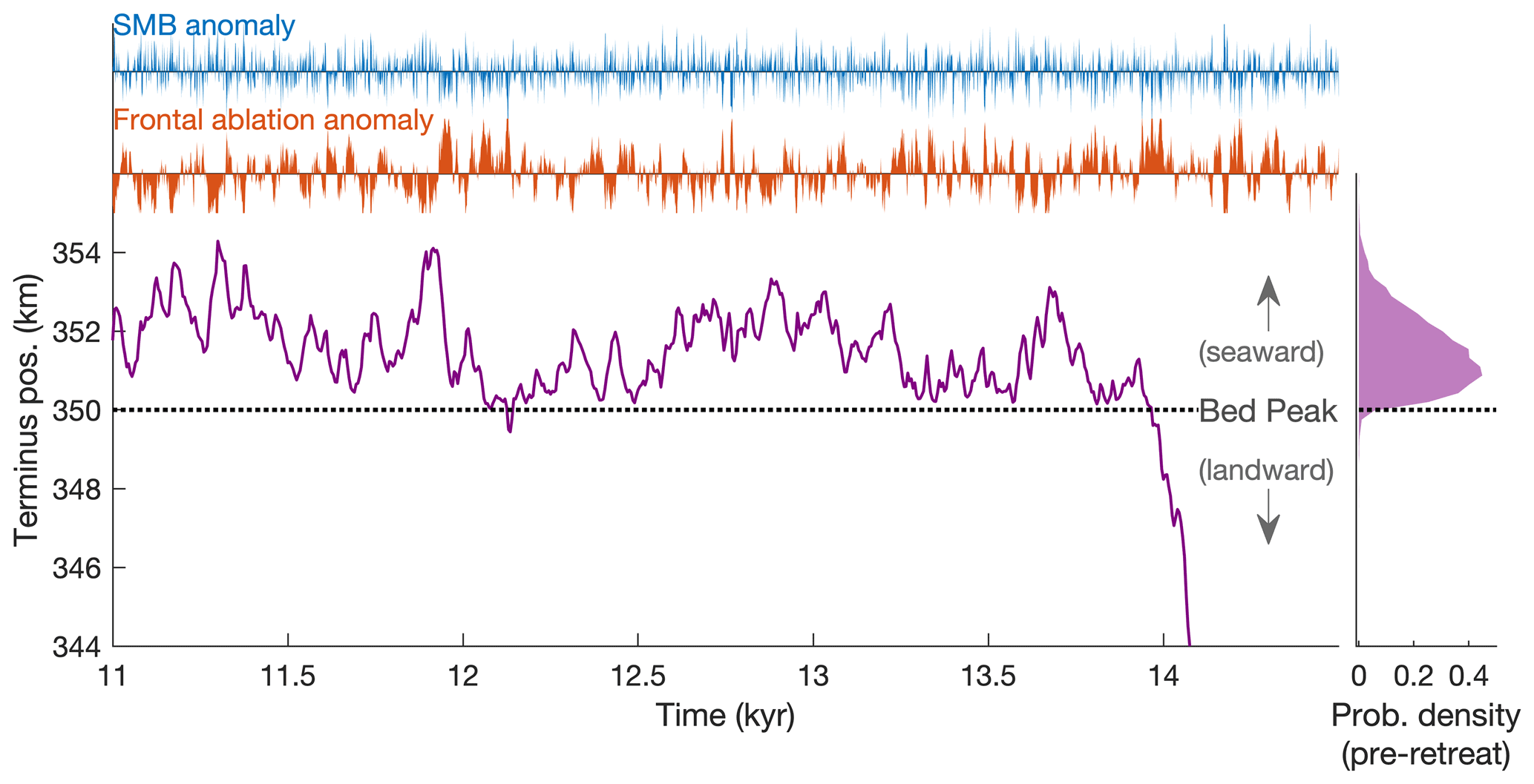
Figure 2A synthetic glacier's response to stochastic variability, when the terminus is near a peak in bed topography. Normalized climate anomalies are shown on the upper axes, and grounding-line fluctuations are below. Dashed line indicates the location of the bed peak. A long period of stable, stationary fluctuations precedes unstable retreat off of the bed peak. The histogram (right) shows the probability distribution of stable fluctuations.
Figure 2 shows a single realization of stochastic SMB and frontal ablation forcing (the latter with σFA=12 m yr−1) and the response from the idealized glacier shown in Fig. 1. The grounding line fluctuates in a roughly 4 km range on the seaward side of the bed peak for over 14 kyr before retreating permanently from the peak due to one particularly persistent (but random) anomaly in both frontal ablation and SMB. Retreat continues over several centuries until the terminus reaches a new stable mean state several tens of kilometers inland (not shown), consistent with the marine-ice-sheet instability. This simulation illustrates the basic null hypothesis for attribution: a sustained retreat from a bed peak initiated purely by natural variability. It also highlights the stochastic nature of such retreats: the glacier fluctuates for a long time in close proximity to the topographic threshold, before permanently retreating. The frontal ablation and SMB anomalies that triggered retreat occurred purely by chance in the sequence of stochastic forcing.
2.3 Ensemble framework
The stochastic nature of noise-driven retreat from a bed peak (Fig. 2) suggests that for attribution, it may be more productive to consider such retreats as discrete events rather than trends, as well as to focus on their likelihood rather than their total magnitude, which is set largely by bed topography. Our method is to run large ensembles (i.e., collections) of simulations with the glacier model, in which each simulation is forced with an independent realization of random climate variability drawn from the same distribution. This assumes that the statistics of the forcing variability are related to constant physical characteristics within the climate system, but the particular sequence of anomalies is fundamentally random. Because any realization of such climate variability is equally plausible, the ensemble thus provides a statistical population from which we can estimate the likelihood of a particular event, such as a sustained retreat from the bed peak. We refer to these ensembles as “aleatory” ensembles because the only difference between members is the realization of random forcing.
Unless otherwise indicated, we assess glacier retreats within an experimental interval of 150 years, corresponding to the approximate time frame of significant anthropogenic forcing (e.g., IPCC, 2021). Within this interval, we count ensemble members with termini that start seaward of the bed peak and the retreat more than 4 km behind the bed peak. This threshold corresponds to the inland extent of the retrograde bed (Fig. 1), so it is a reasonable indicator that the retreat is due to a loss of terminus stability and that the terminus will continue retreating (indeed, this is observed in longer simulations). However, since stability thresholds can be ambiguous for transient glacier states (Sergienko and Wingham, 2021; Robel et al., 2022), we refer to retreats exceeding this threshold as rapid and sustained retreats. The threshold is within the range of many observations of retreats from bed peaks (e.g., Catania et al., 2018; Wood et al., 2018). For attribution assessments on real glaciers, the threshold for what counts as a retreat within ensemble simulations would be informed by the observed retreat extent. We return to the question of defining retreats in the discussion section.
Rather than starting all simulations with a strictly steady-state glacier, we initialize simulations with a 250-year period of stochastic forcing. This is necessary because of noise-induced drift that occurs at the onset of stochastic forcing due to nonlinearities in ice dynamics (e.g., Robel et al., 2018). Indeed, we find that the steady-state grounding line position is closer to the bed peak than the long-term mean under noisy forcing, slightly enhancing the likelihood at the beginning of simulations initiated from a steady state (see Supplement, Figs. S4–S5).
From each aleatory ensemble, we estimate the probability of sustained retreat as the number of retreats within the 150-year experimental interval (as defined above) divided by the total number of simulations with termini seaward of the peak at the beginning of the interval. That is, we are fundamentally focusing on a conditional probability of industrial-era retreat (i.e., conditioned on the glacier not having already retreated). We ran several long ensemble simulations to assess how this conditional probability varies in time and find it to be fairly stable after the noise-induced drift decays, though with some additional caveats at millennial timescales (see Supplement, Fig. S5). We assess the role of anthropogenic forcing by comparing the probability of retreat between an ensemble with constant mean climate and another ensemble with an anthropogenic trend in the mean climate added to all members (Sect. 4).
The aleatory ensembles are the key tools of the attribution framework we propose and are necessary because of the fundamentally chaotic nature of climate variability. A few previous studies have analyzed aleatory ensembles for ice-sheet dynamics, focusing on uncertainty in future response (Tsai et al., 2017; Robel et al., 2019; Tsai et al., 2020), but the present study is the first application to the question of attribution. However, a different category of ensemble methods also exists for quantifying “epistemic” uncertainty in the design or parameter choices within the model. In principle, such epistemic uncertainty can be reduced by adding observational or theoretical constraints, whereas aleatoric uncertainty is irreducible due to the lack of predictability of climate variability. These ensemble methods have recently seen wider use for ice-sheet models. Examples include intercomparison projects targeting structural differences between models (e.g., ISMIP6; Nowicki et al., 2016), perturbed-parameter ensembles (e.g., Applegate et al., 2012; Aschwanden et al., 2019; Nias et al., 2019; DeConto et al., 2021), and ensembles of synthetic subglacial topography (MacKie et al., 2021). We also employ ensemble methods in this broader epistemic category. In the next section, we assess the sensitivity of the probability of retreat to several key parameters by running aleatory ensembles over a range of parameter perturbations (note that this means two layers of ensemble design over two different types of uncertainty). Finally, we also consider an ensemble of different bed topographies (Sect. 5) in order to investigate attribution in the context of a regional population of heterogeneous glaciers.
We note again that the synthetic geometries and climate parameters we use are closer in scale to marine-terminating glaciers in Greenland than Antarctica. However, the principles of the ensemble attribution framework constitute a general approach for assessing glacier variability and retreats near topographic thresholds. These methods could thus be applied to other marine-terminating glaciers in a wide range of contexts.
The basic mechanism of glacier retreat on retrograde slopes is well established, and previous modeling studies have investigated controls and thresholds for retreat (e.g., Nick et al., 2009; Enderlin et al., 2013; Parizek et al., 2013; Catania et al., 2018), as well as factors that enhance stability (e.g., Gudmundsson et al., 2012; Pegler, 2018; Gomez et al., 2015; Robel et al., 2022). However, few studies have systematically investigated sustained retreats driven by stochastic climate variability (with some exceptions, see Mulder et al., 2018; Robel et al., 2019). We thus begin by investigating controls on noise-driven retreat before turning to the question of anthropogenic forcing.
In the single simulation shown in Fig. 2, stable fluctuations extend right up to the bed peak before sustained retreat. Despite the instability associated with retrograde slopes, glacier termini near relatively steep bed peaks can be very stable to perturbations (Robel et al., 2022). Ultimately, for attribution, we need to know how stable glaciers are with respect to natural variability, and we can use aleatory ensembles to assess this. We first consider two different 1000-member ensemble experiments, both with a bed-peak height of 94 m. The first ensemble is run with frontal ablation variability of σFA=15 m yr−1 and contains only four ensemble members that produce sustained retreat (Fig. 3b). This is consistent with the long wait time for retreat in Fig. 2. Note that some simulations are excluded under the condition of only considering those with termini landward of the peak at t=0. An ensemble with greater frontal ablation variability (σFA=27 m yr−1) produces a much greater number of sustained retreats (Fig. 3b), with a retreat probability of approximately 18 % in 150 years. Note that the ensemble size is further reduced in Fig. 3b because more members produce retreat during the spinup period. These two cases illustrate how large ensembles can be used to estimate the probability of retreat under internal climate variability but also that the estimated probability is sensitive to model assumptions, including the statistics of the climate variability.

Figure 3Probability of sustained retreat driven by stochastic variability. (a) An aleatory ensemble experiment with frontal ablation variability of σFA=15 m yr−1. Only four simulations (red) produce sustained retreat behind the location of the bed peak (black). Sustained retreat is defined here as retreating past the deepest part of the trough at 346 km (blue). (b) An ensemble subject to stronger variability (σFA=27 m yr−1), in which approximately 18 % of simulations produce sustained retreat. (c) Retreat probabilities for a range of bed-peak heights (circles), SMB (triangles), and friction coefficients (downward triangles). Symbols are colored by the range in σFA. Arrows indicate the ensembles shown in (a) and (b).
3.1 Which model parameters affect the probability of rapid retreat?
With multiple uncertain parameters that must be prescribed in any model, it is important to consider how sensitive retreat probabilities estimated from an ensemble will be to such uncertainties. We assess this by running groups of aleatory ensembles, where each ensemble has slightly different model parameter values (model parameters are still identical between the 1000 simulations within a single aleatory ensemble). We perturb the bed peak height (from 88 to 100 m), the mean interior SMB (64 to 71 cm yr−1), and the friction coefficient (reductions of 2 % to 22 % from the default value). We vary only one parameter at a time, but for each group of perturbations, we also apply three levels of frontal melt variability (σFA of 15, 21, and 27 m yr−1).
Figure 3c shows the retreat probabilities of 51 ensembles, each with 1000 members, across this parameter space. Retreat probabilities are plotted against the distance between the initial steady-state terminus position (before being forced by climate variability) and the bed peak. Although the steady-state terminus position is not strictly the same as the time mean of fluctuations (see Supplement, Fig. S4; Robel et al., 2018), it still provides a metric for comparing how these parameter perturbations affect how close the system is to the topographic threshold. From Fig. 3c, we can see that the probability of rapid retreat varies primarily along two dimensions; the proximity of the glacier terminus to the bed peak and the magnitude of noisy forcing. Regardless of which model parameter is changed (besides σFA), the probability of retreat ultimately collapses onto curves that are solely a function of the steady-state distance of the terminus from the bed peak (i.e., the different colored markers in Fig. 3c). It is possible that parameter perturbations can affect dynamical stability in other ways (e.g., Parizek et al., 2013), but the similarity of these curves for qualitatively different parameters (sliding, mass balance, and bed geometry) indicates that in this case, proximity to the bed peak is the main effect. Similarly, the effect of increasing the climate variability is fairly consistent for a given initial steady state regardless of which glaciological parameters are perturbed to achieve that state.
Setting up attribution experiments for real glaciers will require prescribing multiple uncertain parameters, and the probability of retreat can change quickly across a relatively small range (Fig. 3c). It will thus be important to evaluate how sensitive estimates of retreat probability are to these uncertainties. We note this may also include choices in numerical methods, such as the manner in which frontal ablation is prescribed (see Supplement, Fig. S2). Although there are many parameters to consider, Fig. 3c shows that the priority should be for sensitivity tests to adequately sample the plausible range of mean terminus position prior to retreat and of the magnitude of forcing variability. Both of these key constraints will likely require better observations of glacier state and climate from before the satellite era.
3.2 What causes individual glacier retreats?
Beyond providing a means to estimate the probability of glacier retreat, aleatory ensembles also provide large synthetic datasets that can offer further insight into the process of sustained retreat in the context of climate variability. In Fig. 4 we analyze a 1000-member ensemble, run for 500 years with frontal ablation variability that has σFA=18 m yr−1. We use the standard idealized geometry with a bed peak of 90 m. From this ensemble, we find 375 simulations that retreat more than 4 km, which we will refer to as the “retreat group”. These retreats begin at random times within each simulation. In order to analyze them together, in Fig. 4a we synchronize the time series such that the year 0 corresponds to the last time that the terminus is forward of the bed peak. We conduct the same synchronization for each ensemble member's corresponding time series of frontal ablation forcing so that the anomalies causing retreat are lined up (Fig. 4c). Then, for comparison to the retreat group, we select the simulations that temporarily retreat at least 1 km behind the peak but then recover instead of retreating entirely. These are also synchronized to the onset of retreat (Fig. 4b and d). Comparing the ensemble-mean forcings for both synchronized groups demonstrates that the frontal ablation anomalies that trigger sustained retreat are not systematically larger than those that allow recovery (Fig. 4e). However, they are on average more persistent into the decades following the onset of retreat. Note that in some individual cases visible in panel (c), this persistence is not a continuous excursion but multiple positive anomalies in quick succession.
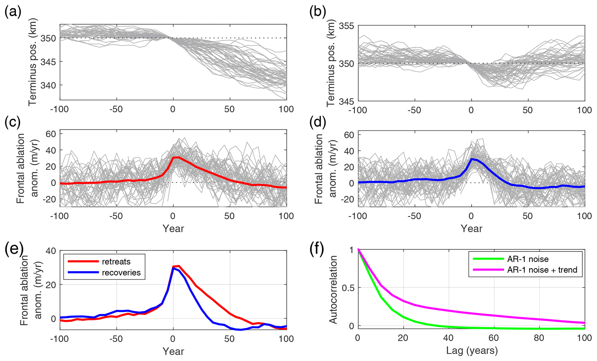
Figure 4Unstable retreats are driven by persistent anomalies in climate forcing. (a) Unstable retreats from a 1000-member ensemble, synchronized to the time that retreat begins (only 50 members shown for clarity). (b) Synchronized members from the same ensemble that retreated >1 km from the bed peak but then recovered. (c) Synchronized frontal ablation anomalies for the retreat group in (a), along with the group mean (red). (d) As for (c) but for the recovery group. (e) Group-mean frontal ablation anomalies plotted together. On average, the key difference between unstable retreats and recoveries is the persistence of the anomalies rather than the maximum at year 0. (f) Autocorrelation function of the AR-1 noise used to simulate frontal ablation anomalies (green) and autocorrelation of the same AR-1 noise plus a 150-year trend of similar magnitude to the variability. A trend will enhance persistence on the multidecadal time frames that set apart the retreat and recovery groups in (e).
The importance of persistent climate anomalies for triggering sustained glacier retreats is related to the timescales of transient ice dynamics. Consider an initial terminus fluctuation driven by anomalous frontal ablation. If the terminus retreats past the bed peak and into deeper water, discharge will increase due to the strong dependence of ice flux on grounding-line thickness (Schoof, 2007). Independent of the initial forcing, this drives dynamic thinning and further retreat (i.e., the marine-ice-sheet instability mechanism begins). These changes are not instantaneous; ice flow near the terminus evolves on multidecadal timescales (Robel et al., 2018), so retreat is reversible if the climate forcing anomaly recovers before significant changes in the inland ice flow occur (Fig. 4b). However, the longer the terminus persists behind the bed peak, the more interior ice is lost to the increased discharge. At some point, dynamic thinning and retreat will proceed to the point where the terminus cannot recover even if the initial forcing reverses, and thus the marine-ice-sheet instability takes over in driving the retreat.
The groups of simulations in Fig. 4 reflect only one aleatory ensemble, in which the time series of forcing variability are drawn from the same statistical distribution. That is, the average persistence of the variability is prescribed, but individual excursions from the mean vary in duration, purely by chance, as would be expected in natural internal climate variability. However, an external forcing trend systematically adds persistence to any time series (Fig. 4f), with a positive trend increasing the time that positive excursions are above the pre-trend mean. We can anticipate that such extra persistence will affect the probability of rapid glacier retreats, as we explore in the next section.
Attribution of observed glacier changes depends on comparing simulations with and without anthropogenic forcing. For individual glaciers, this requires an estimate of the local signature of anthropogenic climate change, which is an attribution challenge itself (e.g., Hegerl et al., 2006). The rate and the time of onset of anthropogenic forcing trends are especially uncertain in the polar regions due in part to a scarcity of long-term instrumental records. We return to this issue in the discussion but proceed here with a synthetic attribution experiment consisting of two possible anthropogenic forcing scenarios (an early onset and late onset), as well as the counterfactual scenario of no anthropogenic forcing (Fig. 5a). Although these are idealized simulations, multiple forcing scenarios give us a way to assess how the timing of anthropogenic climate changes affect attribution for glaciers.
We consider three hypothetical scenarios of ocean forcing over the industrial era (which we take to be 1870–2020 CE): (1) an increase in frontal ablation (ΔFA) of 24 m yr−1 applied as a linear trend over the 150 years, (2) the same increase over only the last 50 years, and the counterfactual scenario of no trend (Fig. 5a). Stochastic anomalies are also added to each scenario, with σFA=18 m yr−1 and a persistence timescale of 10 years. Although not explicitly emulating a particular climate record, this forcing is meant to generally capture the status of climate variables thought to affect ice–ocean interactions. That is, century-scale trends exist (e.g., in ocean temperatures or circulation anomalies), but (multi-)decadal variability is comparable in magnitude (e.g., Straneo et al., 2013; Holland et al., 2019; O'Connor et al., 2021). The values here will give an average signal-to-noise ratio () of about 1.3, which for a single time series is insignificant at 95 % under a one-tailed t test (assuming decadal persistence). However, note that the particular sequence of anomalies in Fig. 5a has a greater apparent trend, purely by chance.
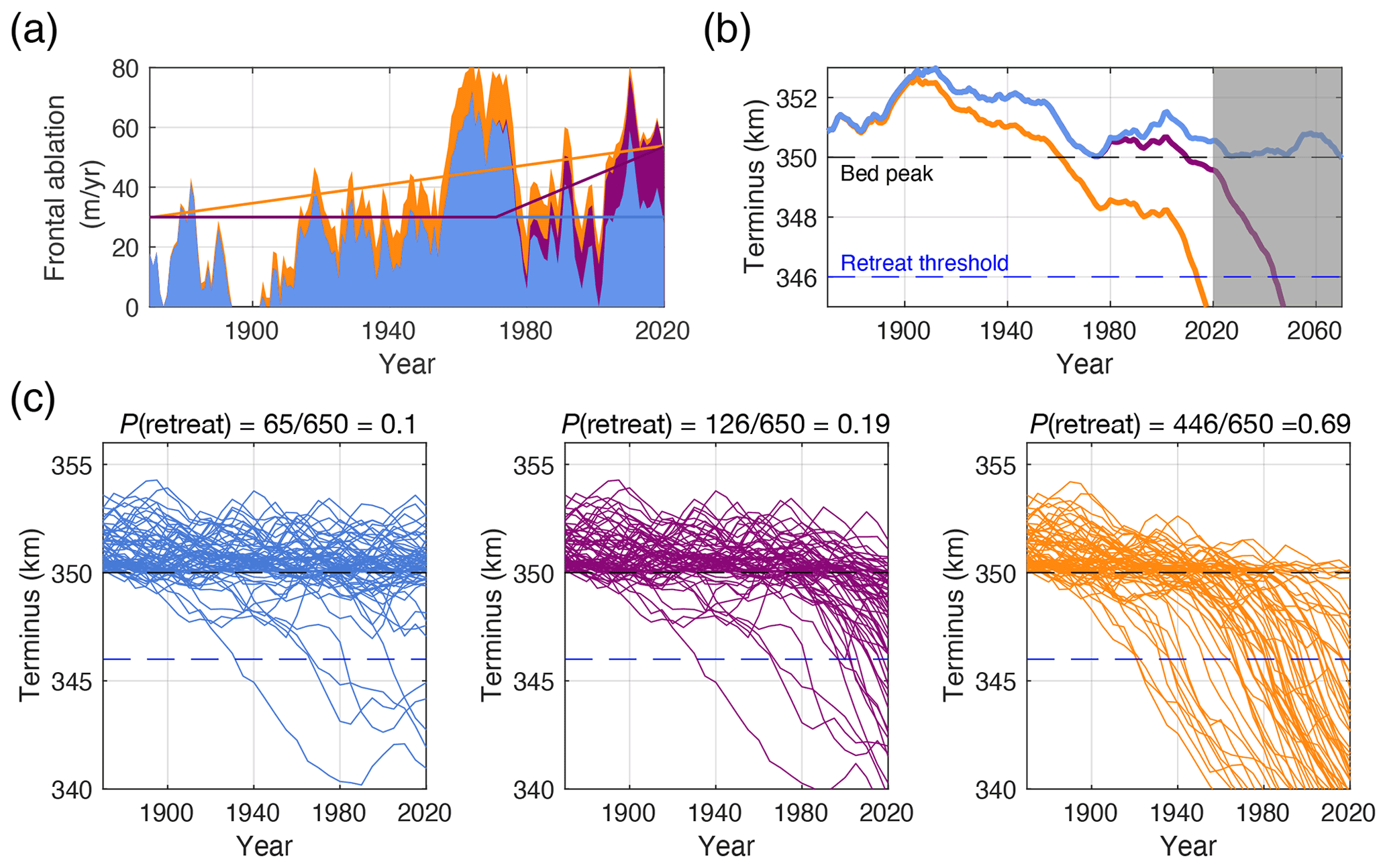
Figure 5The effect of a persistent trend on retreat probability. (a) Three forcing scenarios: no trend (blue), an 80 % increase in frontal melt over 150 years (orange), and a delayed trend of the same total magnitude but over 50 years (purple). Solid lines show the forced trends in frontal ablation, while shaded regions illustrate one realization of stochastic variability added to each scenario. (b) Glacier-terminus responses to the forcing shown in (a). The plot extends past the 150-year experimental interval to show the long-term glacier response to prior forcing (grey shaded); no additional trend is applied after 150 years. (c) Ensemble results (i.e., independent realizations of variability) for these three trend scenarios. For clarity, only 10 % of ensemble members are plotted.
Forcing the synthetic glacier (here with a bed peak of 90 m in height) with the particular frontal ablation anomalies in Fig. 5a, we can see that only the scenarios with an anthropogenic trend drive retreat past the bed peak, though it occurs later for the late-onset trend (Fig. 5b). However, Fig. 5b reflects only one realization of variability, which in this case enhances the overall trend, muddying the interpretation of the retreat. This further motivates ensemble analysis for gaining a more robust understanding for how anthropogenic trends affect the probability of retreat.
For each of the three scenarios, we run 1000-member aleatory ensembles (Fig. 5c). We initialize the experiments and count retreats as described previously. With no anthropogenic trend (left), the probability of retreat is 0.1. In the late-onset scenario (middle), in which the anthropogenic trend is concentrated over the last 50 years, the probability of retreat rises to 0.19, indicating some anthropogenic effect. For the early-onset trend scenario, the probability jumps to 0.69 – a strong anthropogenic effect. We estimate the sampling uncertainty for these probability estimates using standard formulae for ensembles of independent trials (see Supplement). We find standard errors of roughly 0.01–0.03 for the ensembles in Fig. 4, making the effect of the trends far greater than sampling error. However, we stress that this is only one potential source of error, and uncertainties in model parameters could have a larger effect (Fig. 3).
Why is there such a difference between the early-onset and late-onset cases? There are two main effects to consider. First, an external forcing trend makes all positive frontal ablation anomalies more extreme. For the late-onset trend, there is simply a shorter window in which more-positive anomalies affect the probability of retreat. Second, the response timescales of ice dynamics also play a strong role. A glacier's response lags forcing on century timescales, so even if the final magnitudes of the trends are fixed, the earlier-onset trend will push the average terminus position closer to the threshold within the experimental interval. This makes random variability more likely to trigger sustained retreat. We compared these two effects by assessing the probability of retreat after trends of varying duration and found that the lagged dynamic response indeed plays a large role (see Supplement, Fig. S9). This is essentially the same principle that differentiates irreversible retreats from reversible retreats in the absence of a background trend; the glacier response reflects the forcing anomaly integrated over decades or longer (Fig. 4).
Figure 5b illustrates one example of how an earlier-onset trend can be the deciding factor in whether sustained retreat occurs during the experimental interval. In this case, the early-onset trend helps push the glacier beyond the point of recovery when strong frontal ablation anomalies occur in the middle of the simulation (Fig. 5a). We extend the simulations an additional 50 years with no additional trend (shaded), and this shows that the late-onset trend does eventually drive a sustained retreat, but it begins during a later phase of positive random anomalies. We also note the frontal ablation trend also drives sustained retreat in the absence of any variability (not shown), although in such a case it does not reach the 4 km retreat threshold within 150 years. Although sustained retreat is committed even in simulations that do not count as rapid retreats, attribution focuses on the probability of having already observed rapid retreat.
The key takeaway is that a long-term anthropogenic trend, even if it is weak compared to the noise, can significantly increase the probability of unstable retreats within a given time frame. A higher probability of retreat is expected for trends with a longer duration or larger magnitude (see Supplement for additional forcing scenarios). The attribution of observed retreats can be framed around such increases in probability. However, a statistically weak forcing trend is also an uncertain trend, so defining the counterfactual “no forcing” scenario based on observations is a key challenge here. Figure 5 demonstrates that the onset of forcing is an important consideration due to the typical response times of ice dynamics. Multiple ensembles could be run to provide bounds on attribution that are consistent with uncertainties in the anthropogenic forcing. We return to this issue in the discussion section.
So far, we have focused on how to frame attribution for the observed retreat of a single glacier. However, especially in Greenland, groups of glaciers have retreated concurrently within regions and across the entire ice sheet (Murray et al., 2015; King et al., 2018), although with heterogeneity in retreat duration and extent between individual glaciers (Catania et al., 2018). Moreover, total Greenland Ice Sheet mass loss depends on the behavior of many marine-terminating glaciers, which would need to be considered for attributing ice-dynamic contributions to sea-level rise. We therefore consider how attribution might be framed for a population of glaciers. Although there are several mechanisms that may cause heterogeneous glacier responses (e.g., local geometry, catchment size, fjord hydrography, basal hydrology), we focus here solely on variations in bed topography in order to demonstrate the attribution framework. The synthetic glaciers we present below thus do not represent the full spectrum of glaciers that could be found in a region, though similar experiments could be conducted in a more complex ice-sheet model including these other factors.
At regional scales, local topography can explain much of the variation in the magnitudes of terminus retreats (Catania et al., 2018). Similarly, we expect that the pre-retreat distance between glacier termini and bed peaks would vary among individual glaciers and with it the likelihood of rapid retreat (as shown in Fig. 3). Such glacier-to-glacier variation in the thresholds for rapid retreat may make attribution for glacier populations more statistically robust since it could be framed in terms of the fraction of glaciers within a region that retreat rather than the probability of retreat for a single glacier, which may be strongly sensitive to coincidental alignments of random variability and bed topography.
Subglacial topography is known to have self-similar properties over a wide range of length scales (e.g., Jordan et al., 2017). To emulate these characteristics, we use a MATLAB function for generating random surfaces with prescribed self-similarity characteristics (Kanafi, 2021). We consider an initial population of 200 glaciers with random bed topographies. For each glacier, we start with a gentle prograde bed slope () and then superimpose topographic variations, unique to each glacier, beyond x=200 km. Topography is generated with a fractal dimension of 0.5 and root-mean-square variation of 80 m, which are realistic statistics describing variations in bed topography in Greenland (Jordan et al., 2017), although we note that the assumption of random variations may fail to capture non-random aspects of topography unique to terminus regions. To avoid aliasing as the glacier model's numerical grid varies in time, we smooth the bed profiles with a 30 m running mean filter and also refine the numerical grid in the region of topographic variability to approximately 1 km (the model's grid resolution remains <0.1 km for ∼6 km upstream of the terminus). This smoothing enhances numerical stability of the model, but we expect it has little impact on the locations of actual glacier stability since it is much finer than the ice thickness (e.g., Gudmundsson, 2003).
To generate a self-consistent glacier geometry on each synthetic topography, we start with a terminus position beyond the random topographic variations (which aids initial numerical convergence) and then reduce SMB so that the terminus retreats toward a new equilibrium within the variable topography. We allow 5000 years for this adjustment, imposing frontal ablation variability throughout (identical for all glaciers). Some glaciers evolve quickly to new stable positions (e.g., Glacier 21; Fig. 6), while others exhibit multiple punctuated retreats over several millennia (e.g., Glacier 28; Fig. 6), depending on their individual bed topographies. The end result is a population of glaciers with a spread of terminus positions grounded on a variety of prograde slopes and bed peaks (Fig. 6b). We discard glaciers that have less than 10 km of variable topography inland of the terminus at t=5000 years (light grey in Fig. 6a), leaving a population of 177 glaciers (dark grey in Fig. 6a). Although this may bias the population of considered glaciers towards stability, the number of excluded glaciers is relatively small (n=23).
We then use the glacier states at t=5000 years as the initial conditions for a synthetic attribution experiment. Of these, there is a wide distribution in the distance between the terminus and the nearest local topographic peak (Fig. 6c). The majority are within 5 km of a peak; however, peaks are defined simply as local maxima of the smoothed self-affine topography. As a result, peaks range from a few tens to several hundreds of meters in height (compared to their nearest troughs) and thus may provide different degrees of stability. This spinup should not be interpreted as a reconstruction of glacier behavior over the last several millennia; it is simply a procedure to yield a population of quasi-steady termini on random topographies.
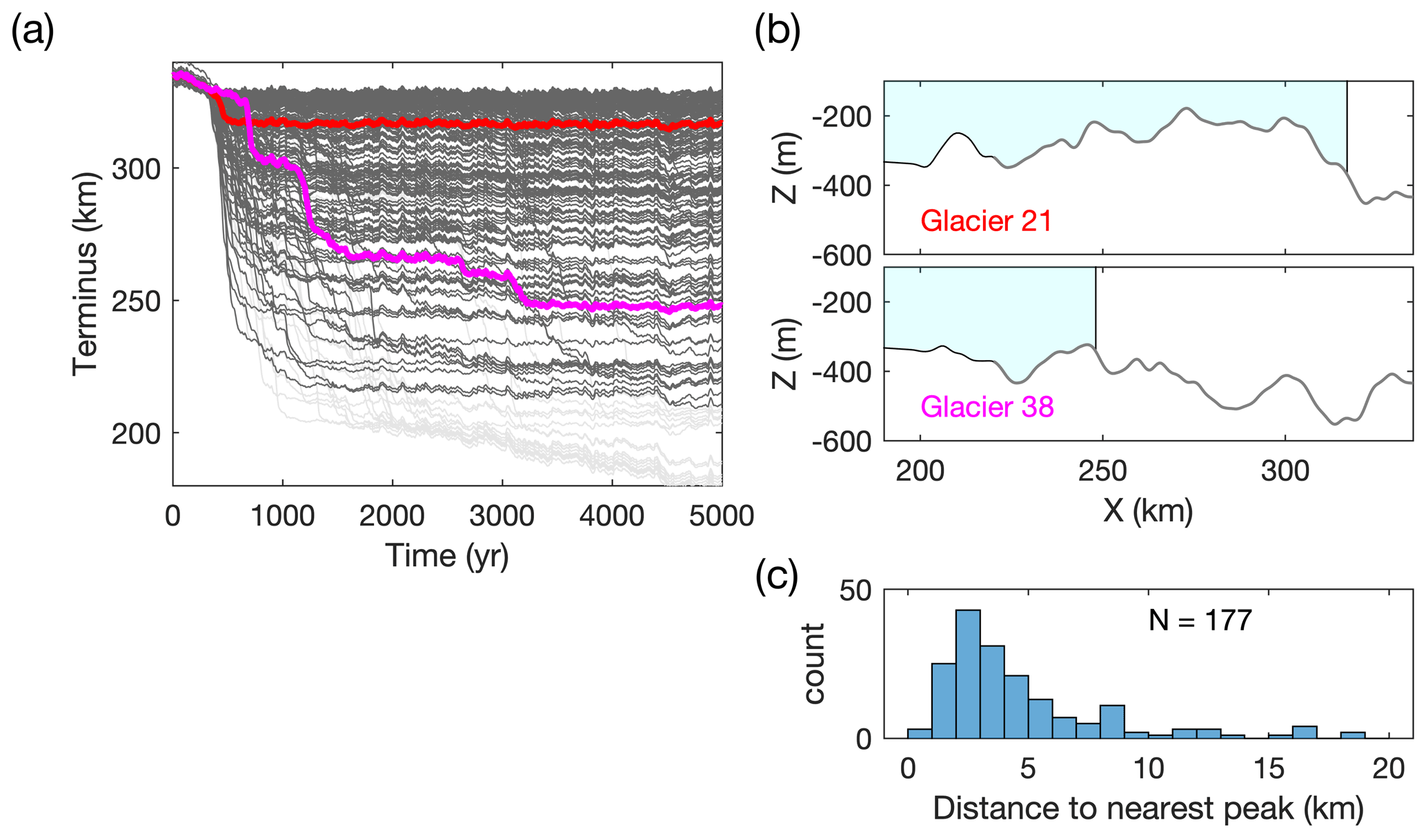
Figure 6Simulating a population of glaciers with randomly generated bed topographies. (a) Transient spinup to find quasi-stable initial conditions in random topographies. Two glaciers are highlighted (red and magenta) to illustrate the range of different retreat histories. Light-grey lines indicate glaciers excluded from subsequent analyses. (b) Topographic profiles and terminus position at the end of the spinup for the two glaciers highlighted in (a). Note the very different topography inland of the terminus. Glacier ice is colored blue. (c) Distribution of 177 terminus positions at t=5000 years with respect to the nearest bed peak.
We now assess the role of an external forcing trend over a 150-year interval in driving retreat within this population of glaciers. Whereas the transition from stable to unstable terminus positions was simplified by the single bed peak in previous experiments (Fig. 1), transitions can be less obvious with topographic complexity at smaller scales, especially when a glacier is fluctuating in response to climate variability. Rather than focusing strictly on dynamical stability, which can be very difficult to assess from observations (Robel et al., 2022), we simply set a threshold of 2 km net retreat over the experiment to consider a glacier as “retreated”. This choice is arbitrary, but our purpose is to have a common retreat threshold for the population so that the number of rapid retreats can be compared between forcing scenarios. We show qualitatively similar results with different threshold values in the Supplement.
We force each glacier in the population with the same frontal ablation anomalies in order to mimic regionally coherent climate variability. This neglects a number of factors that can cause ocean forcing to vary widely between individual glaciers (e.g., Straneo et al., 2011; Wood et al., 2021), but our focus remains on simplified experiments to illustrate attribution – here with a variety of topographies. With stochastic variability and no external trend, termini fluctuate coherently, though by slightly different amounts depending on how different bed geometries modulate terminus fluctuations (Fig. 7a). However, only one glacier shows a net retreat of >2 km. In contrast, with a frontal ablation trend of 30 m yr−1 over 150 years (and the same stochastic anomalies), there is an overall retreat trend for the population, with the majority retreating >2 km over the latter part of the simulation (Fig. 7b).
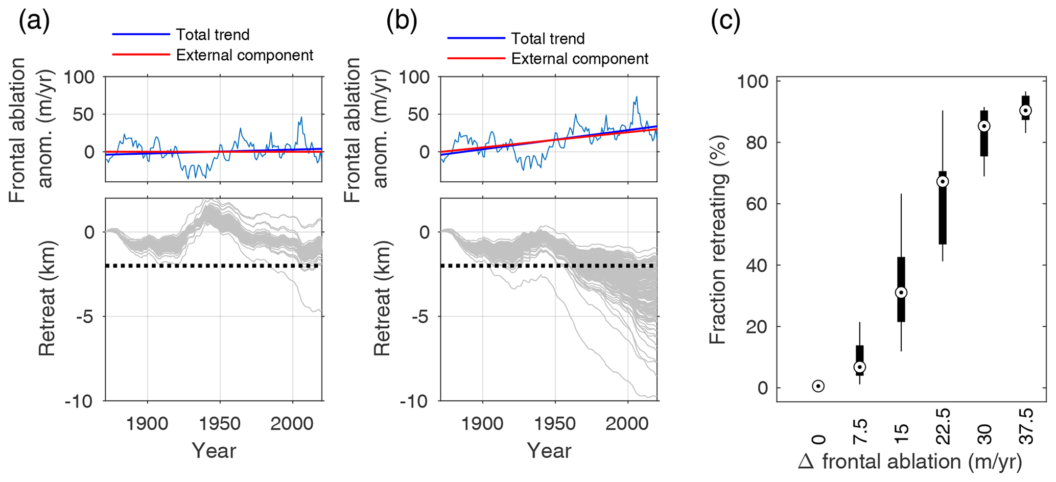
Figure 7Synthetic attribution experiment for a population of glaciers. (a) Terminus change (relative to year 0) for each glacier, all forced with the same frontal ablation anomalies (σFA=15 m yr−1, top), which have no external forcing trend. The slight overall trend (blue line) is due only to sampling natural variability. Dashed line shows a retreat threshold of 2 km. (b) As for (a) except with an external forcing trend in frontal ablation, increasing 30 m yr−1 over 150 years. (c) Box plot showing proportion of glaciers in the population exceeding the retreat threshold across six external forcing scenarios. “External frontal ablation” refers to the total linear trend over 150 years. For each level of forcing, 20 simulations of the glacier population are run with different realizations of climate variability (i.e., a small aleatory ensemble), with the distribution of retreats indicated with box-and-whisker markers.
The simulations shown in Figs. 7a and 7b show only one realization of random climate anomalies. This means that the number of large retreats (in both scenarios) depends partly on the particular sequence of random anomalies. To illustrate this approach more generally, we run simulations for the same population of 177 glaciers with six levels of anthropogenic trends, using small aleatory ensembles of 20 realizations of variability for each scenario (Fig. 7c). As expected, the number of rapid retreats in the population increases with the magnitude of the frontal ablation trend, but there is a spread depending on whether the stochastic variability enhances or reduces the background trend in the latter part of the simulation. This spread is widest for mid-range forcing scenarios, where glaciers are on average closer to topographic thresholds but where large retreats for many glaciers are still contingent on a contribution from natural variability. With a large enough forcing, however, retreats larger than a given threshold are ubiquitous regardless of the sequence of random variability (Fig. 7c).
Earlier, we showed how a long-term trend primes a single glacier for rapid retreat in the presence of climate variability (Fig. 5). Here, glaciers in the population have different sensitivities and thresholds due to their unique bed topographies. Although an external forcing trend generally increases the number of large retreats, modest forcing may first cause a heterogeneous response by pushing some (but not all) glaciers into a range where random variability may trigger rapid retreat. Some glaciers are simply closer to topographic conditions permitting retreat (e.g., as compared in Fig. 6b). However, the failure of some glaciers to retreat significantly does not necessarily preclude a regional attribution statement. Provided that simulations of many glaciers can be undertaken, attribution could be cast in terms of an increased number of large retreats (or an aggregate metric such as volume loss) compared to the case with no external forcing. Thus, observations of a region in which a substantial fraction of the glaciers retreated would likely be a very strong, statistically robust indicator of an anthropogenic influence since it is nearly impossible for this to happen in the absence of a trend (Fig. 7c).
6.1 Uncertainty in the climate forcing
Our results from large aleatory ensembles show how anthropogenic trends in climate forcing affect the probability of rapid marine-terminating glacier retreat in the presence of bed variations, even when the trend is weak compared to natural climate variability (Fig. 5). The comparison between early- and late-onset trends highlights that a glacier's long-term integration of climate forcing is fundamental to the increased probability of retreat. The early stages of anthropogenic forcing may thus play an important role in an overall attribution assessment. These effects are very clear in the synthetic experiments, in which the difference between ensembles – that is, an anthropogenic climate trend – is simply imposed. However, this trend must ultimately be inferred from observations and models of climate, which is an attribution task of its own. When targeting real glaciers, it will be important to evaluate assumptions about the onset and magnitude of anthropogenic trends built into the model simulations.
What do observations tell us about the onset of climate trends in polar regions? Instrumental records spanning the industrial era are scarce or nonexistent in the vicinity of many glaciers, but a few air-temperature records in Greenland extend over two centuries (e.g., Vinther et al., 2006) and show warming trends since the early 19th century. At a regional scale, the multi-proxy reconstructions of Abram et al. (2016) also show an early (∼1830) onset of surface warming in the Arctic but not the Antarctic. The few long-term ocean records off of Greenland show near-surface (0–40 m) temperature variations roughly correlated with air temperatures (Ribergaard and Buch, 2008), though strong variability obscures the onset of local trends. Additionally, mid-latitude Atlantic waters, a key source of thermal forcing for Greenland's glaciers (e.g., Straneo et al., 2011), have been accumulating heat since the late 19th century (Roemmich et al., 2012). These records do not alone partition natural vs. anthropogenic effects but do provide evidence of early-onset trends.
Comparisons of global climate model simulations with and without anthropogenic greenhouse gas emissions show a significant anthropogenic warming signal beginning in the late 19th century and accelerating in the late 20th century (e.g., Haustein et al., 2017; IPCC, 2021). However, the timing of global-mean temperature changes may not translate directly to the local changes relevant to glaciers. Melt thresholds can add nonlinearity to forcing trends, changing the time of emergence (e.g., Trusel et al., 2018). Transient warming is also slower for ocean variables due to the thermal inertia of the ocean, and localized radiative feedbacks produce further regional variations in surface warming, especially at high latitudes (e.g., Armour et al., 2013). Additionally, the spatiotemporal signature of some forcing agents is relevant at high latitudes. For example, anthropogenic aerosols had an outsized effect in the Arctic and North Atlantic in the 20th century, and several studies have concluded that they effectively canceled the greenhouse-gas forcing in the mid-20th century in the Arctic (e.g., Fyfe et al., 2013; England et al., 2021). This would imply a more step-wise anthropogenic forcing trend, which would be important to account for in attribution experiments. Note that time variations in aerosol forcing also complicate interpretations of Atlantic multidecadal variability (Mann et al., 2020). For glaciers sensitive to this variability, these effects would be important to consider when defining the timescales of stochastic forcing in model experiments.
Despite these challenges, it is still possible to get a sense of the external forcing component using output from coupled climate model ensembles. Single-model large ensembles (in which ensemble members differ only due to internal variability) can be used to estimate externally forced trends at any model grid point (e.g., Deser et al., 2012), and unforced simulations are available for comparison. Statistical methods for estimating the forced and internal components in model output and observations also continue to improve (e.g., Mckinnon et al., 2017; Wills et al., 2020).
Our results suggest that assessing uncertainty in the anthropogenic component of local climate forcing will be very important for understanding the robustness of attribution statements because of the way glacier dynamics integrate progressive forcing. Ultimately, attribution statements are always made with reference to a world without anthropogenic forcing, which only exists in models. In order for an attribution analysis to provide useful insight, the assumptions about this counterfactual world have to be clearly presented and their limits recognized.
6.2 Initial glacier conditions
Uncertainty in the preindustrial glacier state is also important to consider in attribution studies. We have shown that a glacier's initial proximity to a topographic threshold is a key factor in its probability of retreat (Fig. 3), but few terminus records are available before the satellite era (e.g., Goliber et al., 2021). Moreover, the terminus will have fluctuated due to variability in the preindustrial climate (e.g., Fig. 2), so even if early terminus positions are known, discrete observations still leave some uncertainty in the mean state.
It is worth considering limiting cases and what they would imply for attribution. One limit is a mean preindustrial terminus position far enough from a topographic peak that it is virtually impossible for natural terminus variability to breach the threshold. In this case, an observed retreat from the peak could likely be strongly attributed to external forcing. Note that this would also require a large forced response to drive the terminus toward the peak prior to rapid retreat. The other limit is a terminus position perched right at the peak so that natural variability may quickly drive retreat. We expect it is unlikely to encounter this limit because such a glacier would have already retreated due to past variability in a stationary climate. The likely targets for attribution studies – that is, those glaciers that have retreated from bed peaks during the observational era but for which the anthropogenic role is ambiguous – will fall somewhere between these limits. It will be necessary to test the sensitivity of conclusions in an attribution study to the range of preindustrial conditions compatible with available observations. Fortunately, assumptions about the mean state affect the probability of retreat in the same direction for ensembles with and without trends in forcing (unlike assumptions about the forcing, discussed above). That is, initial conditions closer to a bed peak make retreat more likely whether there is a trend in the forcing or not, but the difference between the two scenarios is still a way to assess the anthropogenic role despite uncertainties in initial conditions. This would also apply to other parameters common to the scenarios with and without trends, such as the magnitude of stochastic climate variability. Nevertheless, improved constraints on pre- or early-industrial-era glacier state remain an important goal for providing context for recent changes. To extend observations of glacier state before satellite or aerial campaigns, trimlines, marine sediments, and bathymetry may offer useful constraints (Andresen et al., 2012; Csatho et al., 2008; Smith et al., 2017).
Finally, it is also worth considering what an ice sheet's long memory of Holocene climate variations implies for the stability of preindustrial termini with respect to bed peaks. An important and broad question remains as to why glacier termini should be near topographic thresholds to begin with. On one hand, it may seem unlikely to find any glaciers near thresholds if there is a non-trivial probability that random variability will eventually drive retreat. On the other hand, glacier termini may be transiently persistent at bed peaks even without long-term stability (Robel et al., 2022). As an ice sheet responds to natural climate variations (at all timescales) and its margin evolves over variable topography, one might expect to find most termini near peaks at any given time. Indeed, we observe a similar condition in our model spinup with synthetic random topographies (Fig. 6), although this was not strictly intended to emulate past climate. It is also important to consider here that glaciers affect their landscape via erosion, sedimentation, and lithostatic deformation, and so topography may not be random with respect to the terminus. For example, proglacial sedimentation or the character of over-deepened topography immediately upstream of the terminus might yield clues as to how persistent termini have been, which could help bound the probability of noise-driven retreat. Investigating these geomorphic processes in the context of climate variability could help refine our view of terminus stability in both the preindustrial and modern climate.
6.3 Defining glacier “retreat”
Our numerical experiments focus on the general phenomenology of rapid marine-terminating glacier retreats in the context of climate variability. Accordingly, we assume certain thresholds for retreat in the simulations. However, for analyses of specific glaciers, it will be necessary to define what aspects of the observed change are the target for attribution, and therefore what counts as reproducing the glacier retreat “event” in simulations. For probabilistic attribution, it is generally the case that the more narrowly an event is defined, the harder it is to attribute to external forcing because fewer simulations will resemble the observation in detail (van Oldenborgh et al., 2021). For example, if bed topography permits sustained retreat for many decades once initiated (i.e., lacking stabilizing topographic features), then the cumulative retreat observed so far depends partly on when retreat was triggered.
The varied timing of terminus retreats in Greenland illustrates this issue. Before the widespread retreats of the last few decades, many marine-terminating glaciers also retreated following rapid Arctic warming in the 1920s and 1930s (Bjørk et al., 2012; Vermassen et al., 2019; Andresen et al., 2012). Some, such as Upernavik and Kangerdlussuaq glaciers, have retreated nearly monotonically through deeper bathymetry since then, although with some variation in the rate of retreat (Khan et al., 2014; Vermassen et al., 2019). For attributing early-onset retreats, one might focus on the full observed change, assessing the number of stochastic simulations that reproduced the full magnitude of observed retreat. This would likely select for stochastic anomalies that trigger retreats early in the simulation, reducing the relative importance of long-term trends. Alternatively, one could take a binary approach, focusing on any sustained retreat over some threshold initiated in the simulation period. This would admit later-onset retreats into the analysis, allowing anthropogenic trends in the forced ensemble to have more effect. However, in such a case, the full magnitude of observed retreat would not necessarily be part of the formal attribution assessment, and this would have to be clearly stated. It is reasonable to hypothesize that retreats triggered early in the industrial era were more contingent on natural climate anomalies compared to more recently initiated retreats. Some glaciers in West Greenland retreated abruptly in the early 2000s and have since stabilized on new bed peaks (Catania et al., 2018), offering very discrete changes that would be potentially easier to define as targets for attribution experiments. Future work might compare these recent retreats against early-onset, more continuous retreats.
These issues illustrate possible tradeoffs associated with defining the target glacier retreat event. Once again, attribution is inherently contingent on the assumptions and framing of the analysis. Choices on how to define the observed change will affect the final quantitative elements of the attribution statement (e.g., how much more likely was a given retreat made by anthropogenic changes). Our main point here is that such choices have to be carefully considered and clearly communicated in future attribution studies.
In this paper, we have proposed a framework for attributing rapid marine-terminating glacier retreats to anthropogenic forcing trends. These glaciers may exhibit threshold behaviors associated with their bed topography, which adds ambiguity to the cause of observed retreats because it is possible for natural climate variability alone to trigger sustained retreat from a bed peak (Fig. 2). Thus, we have proposed framing attribution in terms of the probability of retreat under natural variability, comparing scenarios with and without some anthropogenic forcing signal. The probability of retreat can be estimated using large ensembles of glacier model simulations, each with independent realizations of climate variability (Fig. 3). This approach to attribution is different from an “either-or” question of whether retreats reflect variability or trends. Focusing on the likelihood of retreat embraces the role that internal climate variability appears to play in the timing of observed rapid retreats but still provides a way to quantify anthropogenic effects.
We conducted synthetic attribution experiments for single glaciers and for a population of glaciers with different geometries. For a single glacier, attribution is based on comparing at least two aleatory ensembles: one (or more) with an anthropogenic forcing trend common to all members and one with no anthropogenic forcing. For a regional population of glaciers, we would expect variations in how close preindustrial termini were to topographic thresholds. Using a population of synthetic random topographies, we showed that forcing trends increase the fraction of glaciers in the population that cross topographic thresholds and undergo major retreats (Fig. 7). This could thus be a metric for regional attribution in settings where observed retreats have been heterogeneous.
The results from ensembles are sensitive to topographic boundary conditions, glacier-dynamical parameters, and the statistics of the climate forcing. Our sensitivity tests suggest that these factors affect the probability of retreat along two key dimensions: the glacier's proximity to a topographic threshold and the magnitude of its natural fluctuations in climate forcing (Fig. 3c). It will be critical to assess the sensitivity of attribution statements to parameter uncertainty, but it may be sufficient to test along the plausible range of these two dimensions rather than conducting an exhaustive parameter sweep across many more dimensions. This may help in devising more efficient sampling strategies for uncertainty quantification studies using models that are more computationally expensive compared to the relatively simple model used here.
Most importantly, these ensemble experiments show that even modest anthropogenic forcing trends could have a large effect on the probability of retreat, especially on century and longer timescales. Our simulations are idealized, but we expect this is a robust result because it reflects the fundamental timescales over which the ice dynamics integrate and respond to climate variability and trends (Robel et al., 2018; Christian et al., 2020). Recent analysis of mountain glacier retreat has also noted the importance of ice-dynamic response times in reasoning about attribution (Roe et al., 2017). For marine-terminating glaciers, it is important to consider century-scale responses even when rapid retreats appear to coincide with short-term climate fluctuations. The total effect of a long-term climate trend is not limited to making short-term climate anomalies more extreme but also includes the preceding decades of forcing, which gradually push the terminus closer to the topographic threshold than it otherwise would be. As a result, the probability of retreat in a given period depends strongly on the onset and duration of external forcing (Fig. 5). The takeaway is that there are firm physical grounds for hypothesizing that a century or more of anthropogenic forcing has affected the probability of rapid terminus retreats. A probabilistic framing, enabled by ensemble simulations, is a way to quantify an anthropogenic effect even if individual retreats coincide with natural climate fluctuations.
As discussed in the previous section, uncertainties in a glacier's preindustrial position and in the onset of anthropogenic forcing pose fundamental challenges for attribution, as do uncertainties in key physical processes such as calving, submarine melt, and glacier sliding. Despite these gaps, our view is that sufficient mechanistic understanding and observational constraints exist to motivate ensemble-based attribution assessments on well-observed glaciers. In light of these uncertainties, it may be necessary to test over a range of plausible assumptions about glaciological processes and climate forcing that are consistent with observed retreats. An overall assessment would ideally combine results from this range according to our confidence in each assumption (e.g., Shepherd, 2021).
A logistical challenge to confront is the computational cost associated with large ensemble simulations. We propose that a hierarchical approach may be a way forward. Many thousands of simulations are feasible for 1-D models as we have used here. These can be used to explore a wide parameter space, including different assumptions about initial and boundary conditions. These insights can then help constrain the use of 2-D models that will capture the key geometric controls. Large aleatory ensemble simulations have recently been run using state-of-the-art models (Robel et al., 2019), so we expect that the feasibility of their application to attribution studies will only continue to improve in the coming years.
Even if attribution statements have large uncertainty bounds at first, pursuing such studies may still clarify remaining challenges and offer insights into glacier variability, just as the broader pursuit of attribution in climate science has uncovered insights about climate variability and sensitivity. The ability to make quantitative assessments about the role of anthropogenic forcing is an important benchmark in the study of natural systems. Formal assessments would help focus discussion of recent and ongoing cryospheric change both within the scientific community and in the public.
Code for the core glacier model is available as a persistent Zenodo repository at https://doi.org/10.5281/zenodo.5245271 (Robel, 2021). Additional code for the ensemble analysis within this study, as well as model output and scripts to recreate figures, is also available as a persistent Zenodo repository at https://doi.org/10.5281/zenodo.6525750 (Christian, 2022).
Model output is available at a persistent Zenodo repository at https://doi.org/10.5281/zenodo.6525750 (Christian, 2022).
The supplement related to this article is available online at: https://doi.org/10.5194/tc-16-2725-2022-supplement.
JEC, AAR, and GC designed the study and interpreted results. JEC conducted the analyses and wrote the manuscript with input from AAR and GC.
The contact author has declared that none of the authors has any competing interests.
Publisher's note: Copernicus Publications remains neutral with regard to jurisdictional claims in published maps and institutional affiliations.
John Erich Christian was supported by a postdoctoral fellowship from the University of Texas Institute for Geophysics, as well as NSF Office of Polar Programs Grant 1947882. Computing resources were provided by the Partnership for an Advanced Computing Environment (PACE) at the Georgia Institute of Technology, Atlanta. We thank Ziad Rashed and Vincent Verjans for insightful discussions and feedback, as well as Jeremy Bassis and an anonymous reviewer for thoughtful comments that helped us improve the manuscript.
This research has been supported by the University of Texas at Austin (Institute for Geophysics postdoctoral fellowship) and the NSF Office of Polar Programs (grant no. 1947882).
This paper was edited by Alexander Robinson and reviewed by Jeremy Bassis and one anonymous referee.
Abram, N. J., McGregor, H. V., Tierney, J. E., Evans, M. N., McKay, N. P., Kaufman, D. S., Thirumalai, K., Martrat, B., Goosse, H., Phipps, S. J., Steig, E. J., Kilbourne, K. H., Saenger, C. P., Zinke, J., Leduc, G., Addison, J. A., Mortyn, P. G., Seidenkrantz, M. S., Sicre, M. A., Selvaraj, K., Filipsson, H. L., Neukom, R., Gergis, J., Curran, M. A., and Gunten, L. V.: Early onset of industrial-era warming across the oceans and continents, Nature, 536, 411–418, https://doi.org/10.1038/nature19082, 2016. a
Andresen, C. S., Straneo, F., Ribergaard, M. H., Bjørk, A. A., Andersen, T. J., Kuijpers, A., Nørgaard-Pedersen, N., Kjær, K. H., Schjøth, F., Weckström, K., and Ahlstrøm, A. P.: Rapid response of Helheim Glacier in Greenland to climate variability over the past century, Nat. Geosci., 5, 37–41, https://doi.org/10.1038/ngeo1349, 2012. a, b, c, d
Andresen, C. S., Kjeldsen, K. K., Harden, B., Nørgaard-Pedersen, N., and Kjær, K. H.: Outlet glacier dynamics and bathymetry at Upernavik Isstrøm and Upernavik Isfjord, North-West Greenland, Geol. Surv. Den. Greenl., 31, 79–82, https://doi.org/10.34194/geusb.v31.4668, 2014. a
Applegate, P. J., Kirchner, N., Stone, E. J., Keller, K., and Greve, R.: An assessment of key model parametric uncertainties in projections of Greenland Ice Sheet behavior, The Cryosphere, 6, 589–606, https://doi.org/10.5194/tc-6-589-2012, 2012. a
Armour, K. C., Bitz, C. M., and Roe, G. H.: Time-Varying Climate Sensitivity from Regional Feedbacks, J. Climate, 26, 4518–4534, https://doi.org/10.1175/JCLI-D-12-00544.1, 2013. a
Aschwanden, A., Fahnestock, M. A., Truffer, M., Brinkerhoff, D. J., Hock, R., Khroulev, C., Mottram, R., and Khan, S. A.: Contribution of the Greenland Ice Sheet to sea level over the next millennium, Sci. Adv., 5, eaav9396, https://doi.org/10.1126/sciadv.aav9396, 2019. a
Bjørk, A. A., Kjær, K. H., Korsgaard, N. J., Khan, S. A., Kjeldsen, K. K., Andresen, C. S., Box, J. E., Larsen, N. K., and Funder, S.: An aerial view of 80 years of climate-related glacier fluctuations in southeast Greenland, Nat. Geosci., 5, 427–432, https://doi.org/10.1038/ngeo1481, 2012. a, b
Catania, G. A., Stearns, L. A., Sutherland, D. A., Fried, M. J., Bartholomaus, T. C., Morlighem, M., Shroyer, E., and Nash, J.: Geometric Controls on Tidewater Glacier Retreat in Central Western Greenland, J. Geophys. Res.-Earth Surf., 123, 2024–2038, https://doi.org/10.1029/2017JF004499, 2018. a, b, c, d, e, f, g
Catania, G. A., Stearns, L. A., Moon, T. A., Enderlin, E. M., and Jackson, R. H.: Future Evolution of Greenland's Marine-Terminating Outlet Glaciers, J. Geophys. Res.-Earth Surf., 125, 2, https://doi.org/10.1029/2018JF004873, 2020. a
Christian, J. E.: Marine-terminating-glacier stochastic retreat (release of code for publication), Zenodo [code], https://doi.org/10.5281/zenodo.6525750, 2022. a, b
Christian, J. E., Robel, A. A., Proistosescu, C., Roe, G., Koutnik, M., and Christianson, K.: The contrasting response of outlet glaciers to interior and ocean forcing, The Cryosphere, 14, 2515–2535, https://doi.org/10.5194/tc-14-2515-2020, 2020. a, b, c
Cook, A. J., Vaughan, D. G., Luckman, A. J., and Murray, T.: A new Antarctic Peninsula glacier basin inventory and observed area changes since the 1940s, Antarct. Sci., 26, 614–624, https://doi.org/10.1017/S0954102014000200, 2014. a
Csatho, B., Schenk, T., der Veen, C. J. V., and Krabill, W. B.: Intermittent thinning of Jakobshavn Isbræ, West Greenland, since the Little Ice age, J. Glaciol., 54, 131–144, https://doi.org/10.3189/002214308784409035, 2008. a
DeConto, R. M., Pollard, D., Alley, R. B., Velicogna, I., Gasson, E., Gomez, N., Sadai, S., Condron, A., Gilford, D. M., Ashe, E. L., Kopp, R. E., Li, D., and Dutton, A.: The Paris Climate Agreement and future sea-level rise from Antarctica, Nature, 593, 83–89, https://doi.org/10.1038/s41586-021-03427-0, 2021. a
Deser, C., Phillips, A., Bourdette, V., and Teng, H.: Uncertainty in climate change projections: The role of internal variability, Clim. Dynam., 38, 527–546, https://doi.org/10.1007/s00382-010-0977-x, 2012. a
Dutrieux, P., Rydt, J. D., Jenkins, A., Holland, P. R., Ha, H. K., Lee, S. H., Steig, E. J., Ding, Q., Abrahamsen, E. P., and Schröder, M.: Strong sensitivity of Pine Island ice-shelf melting to climatic variability, Science, 343, 174–178, https://doi.org/10.1126/science.1244341, 2014. a
Enderlin, E. M., Howat, I. M., and Vieli, A.: High sensitivity of tidewater outlet glacier dynamics to shape, The Cryosphere, 7, 1007–1015, https://doi.org/10.5194/tc-7-1007-2013, 2013. a
England, M. R., Eisenman, I., Lutsko, N. J., and Wagner, T. J.: The Recent Emergence of Arctic Amplification, Geophys. Res. Lett., 48, 15, https://doi.org/10.1029/2021GL094086, 2021. a
Fried, M. J., Catania, G. A., Bartholomaus, T. C., Duncan, D., Davis, M., Stearns, L. A., Nash, J., Shroyer, E., and Sutherland, D.: Distributed subglacial discharge drives significant submarine melt at a Greenland tidewater glacier, Geophys. Res. Lett., 42, 9328–9336, https://doi.org/10.1002/2015GL065806, 2015. a
Fyfe, J. C., Salzen, K. V., Gillett, N. P., Arora, V. K., Flato, G. M., and McConnell, J. R.: One hundred years of Arctic surface temperature variation due to anthropogenic influence, Sci. Rep.-UK, 3, 2645, https://doi.org/10.1038/srep02645, 2013. a
Fyke, J. G., Vizcaíno, M., and Lipscomb, W. H.: The pattern of anthropogenic signal emergence in Greenland Ice Sheet surfacemass balance, Geophys. Res. Lett., 41, 6002–6008, https://doi.org/10.1002/2014GL060735, 2014. a
Gillett, N. P., Stone, D. A., Stott, P. A., Nozawa, T., Karpechko, A. Y., Hegerl, G. C., Wehner, M. F., and Jones, P. D.: Attribution of polar warming to human influence, Nat. Geosci., 1, 750–754, https://doi.org/10.1038/ngeo338, 2008. a
Goliber, S., Black, T., Catania, G., Lea, J. M., Olsen, H., Cheng, D., Bevan, S., Bjørk, A., Bunce, C., Brough, S., Carr, J. R., Cowton, T., Gardner, A., Fahrner, D., Hill, E., Joughin, I., Korsgaard, N., Luckman, A., Moon, T., Murray, T., Sole, A., Wood, M., and Zhang, E.: TermPicks: A century of Greenland glacier terminus data for use in machine learning applications, The Cryosphere Discuss. [preprint], https://doi.org/10.5194/tc-2021-311, in review, 2021. a
Gomez, N., Pollard, D., and Holland, D.: Sea-level feedback lowers projections of future Antarctic Ice-Sheet mass loss, Nat. Commun., 6, 8798, https://doi.org/10.1038/ncomms9798, 2015. a
Gudmundsson, G. H.: Transmission of basal variability to a glacier surface, J. Geophys. Res.-Sol. Ea., 108, B5, https://doi.org/10.1029/2002jb002107, 2003. a
Gudmundsson, G. H., Krug, J., Durand, G., Favier, L., and Gagliardini, O.: The stability of grounding lines on retrograde slopes, The Cryosphere, 6, 1497–1505, https://doi.org/10.5194/tc-6-1497-2012, 2012. a, b
Hasselmann, K.: Stochastic climate models Part I. Theory, Tellus, 28, 473–485, https://doi.org/10.3402/tellusa.v28i6.11316, 1976. a
Haustein, K., Allen, M. R., Forster, P. M., Otto, F. E., Mitchell, D. M., Matthews, H. D., and Frame, D. J.: A real-time Global Warming Index, Sci. Rep.-UK, 7, 15417, https://doi.org/10.1038/s41598-017-14828-5, 2017. a
Hegerl, G. C., Karl, T. R., Allen, M., Bindoff, N. L., Gillett, N., Karoly, D., Zhang, X., and Zwiers, F.: Climate change detection and attribution: Beyond mean temperature signals, J. Climate, 19, 5058–5077, https://doi.org/10.1175/JCLI3900.1, 2006. a
Holland, D. M., Thomas, R. H., Young, B. D., Ribergaard, M. H., and Lyberth, B.: Acceleration of Jakobshavn Isbr triggered by warm subsurface ocean waters, Nat. Geosci., 1, 659–664, https://doi.org/10.1038/ngeo316, 2008. a
Holland, P. R., Bracegirdle, T. J., Dutrieux, P., Jenkins, A., and Steig, E. J.: West Antarctic ice loss influenced by internal climate variability and anthropogenic forcing, Nat. Geosci., 12, 718–724, https://doi.org/10.1038/s41561-019-0420-9, 2019. a, b, c
Howat, I. M., Joughin, I., Fahnestock, M., Smith, B. E., and Scambos, T. A.: Synchronous retreat and acceleration of southeast Greenland outlet glaciers 2000-06: Ice dynamics and coupling to climate, J. Glaciol., 54, 646–660, https://doi.org/10.3189/002214308786570908, 2008. a
IPCC: Climate Change 2021: The Physical Science Basis. Contribution of Working Group I to the Sixth Assessment Report of the Intergovernmental Panel on Climate Change, edited by: Masson-Delmotte, V., Zhai, P., Pirani, A., Connors, S. L., Péan, C., Berger, S., Caud, N., Chen, Y., Goldfarb, L., Gomis, M. I., Huang, M., Leitzell, K., Lonnoy, E., Matthews, J. B. R., Maycock, T. K., Waterfield, T., Yelekçi, O., Yu, R., and Zhou, B., Cambridge University Press, Cambridge, United Kingdom and New York, NY, USA, in press, https://doi.org/10.1017/9781009157896, 2021. a, b, c, d
Jenkins, A., Dutrieux, P., Jacobs, S., Steig, E. J., Gudmundsson, G. H., Smith, J., and Heywood, K. J.: Decadal Ocean Forcing and Antarctic Ice Sheet Response: LESSONS FROM THE AMUNDSEN SEA, Oceanography, 29, 106–117, 2016. a, b, c
Jordan, T. M., Cooper, M. A., Schroeder, D. M., Williams, C. N., Paden, J. D., Siegert, M. J., and Bamber, J. L.: Self-affine subglacial roughness: consequences for radar scattering and basal water discrimination in northern Greenland, The Cryosphere, 11, 1247–1264, https://doi.org/10.5194/tc-11-1247-2017, 2017. a, b
Joughin, I., Smith, B. E., and Medley, B.: Marine ice sheet collapse potentially under way for the thwaites glacier basin, West Antarctica, Science, 344, 735–738, https://doi.org/10.1126/science.1249055, 2014. a, b
Kanafi, M. M.: Surface generator: artificial randomly rough surfaces, MATLAB Central File Exchange [code], https://www.mathworks.com/matlabcentral/fileexchange/60817-surface-generator-artificial-randomly-rough-surfaces (last access: 7 July 2022), 2021. a
Khan, S. A., Kjeldsen, K. K., Kjær, K. H., Bevan, S., Luckman, A., Aschwanden, A., Bjørk, A. A., Korsgaard, N. J., Box, J. E., van den Broeke, M., van Dam, T. M., and Fitzner, A.: Glacier dynamics at Helheim and Kangerdlugssuaq glaciers, southeast Greenland, since the Little Ice Age, The Cryosphere, 8, 1497–1507, https://doi.org/10.5194/tc-8-1497-2014, 2014. a
Khazendar, A., Fenty, I. G., Carroll, D., Gardner, A., Lee, C. M., Fukumori, I., Wang, O., Zhang, H., Seroussi, H., Moller, D., Noël, B. P., van den Broeke, M. R., Dinardo, S., and Willis, J.: Interruption of two decades of Jakobshavn Isbrae acceleration and thinning as regional ocean cools, Nat. Geosci., 12, 277–283, https://doi.org/10.1038/s41561-019-0329-3, 2019. a
King, M. D., Howat, I. M., Jeong, S., Noh, M. J., Wouters, B., Noël, B., and van den Broeke, M. R.: Seasonal to decadal variability in ice discharge from the Greenland Ice Sheet, The Cryosphere, 12, 3813–3825, https://doi.org/10.5194/tc-12-3813-2018, 2018. a, b
MacKie, E. J., Schroeder, D. M., Zuo, C., Yin, Z., and Caers, J.: Stochastic modeling of subglacial topography exposes uncertainty in water routing at Jakobshavn Glacier, J. Glaciol., 67, 75–83, https://doi.org/10.1017/jog.2020.84, 2021. a
Mann, M. E., Steinman, B. A., and Miller, S. K.: Absence of internal multidecadal and interdecadal oscillations in climate model simulations, Nat. Commun., 11, 49, https://doi.org/10.1038/s41467-019-13823-w, 2020. a
Marzeion, B., Cogley, J. G., Richter, K., and Parkes, D.: Attribution of global glacier mass loss to anthropogenic and natural causes, Science, 345, 919–921, https://doi.org/10.1126/science.1254702, 2014. a
Mckinnon, K. A., Dunn-Sigouin, E., and Deser, C.: An “Observational Large Ensemble” to Compare Observed and Modeled Temperature Trend Uncertainty due to Internal Variability, J. Climate, 30, 7585–7598, https://doi.org/10.1175/JCLI-D-16-0905.s1, 2017. a
Meredith, M., Sommerkorn, M., Cassotta, S., Derksen, C., Ekaykin, A., Hollowed, A., Kofinas, G., Mackintosh, A., Melbourne-Thomas, J., Muelbert, M., Ottersen, G., Pritchard, H., and Schuur, E.: Chapter 3: Polar Regions, in: IPCC Special Report on the Ocean and Cryosphere in a Changing Climate, edited by: Pörtner, H.-O., Roberts, D. C., Masson-Delmotte, V., Zhai, P., Tignor, M., Poloczanska, E., Mintenbeck, K., Alegría, A., Nicolai, M., Okem, A., Petzold, J., Rama, B., Weyer, N. M., Cambridge University Press, Cambridge, UK and New York, NY, USA, 203–320, https://doi.org/10.1017/9781009157964.005, 2019. a, b
Miles, B. W., Stokes, C. R., Vieli, A., and Cox, N. J.: Rapid, climate-driven changes in outlet glaciers on the Pacific coast of East Antarctica, Nature, 500, 563–566, https://doi.org/10.1038/nature12382, 2013. a
Moon, T. and Joughin, I.: Changes in ice front position on Greenland's outlet glaciers from 1992 to 2007, J. Geophys. Res., 113, F02022, https://doi.org/10.1029/2007JF000927, 2008. a
Motyka, R. J., Truffer, M., Fahnestock, M., Mortensen, J., Rysgaard, S., and Howat, I.: Submarine melting of the 1985 Jakobshavn Isbræ floating tongue and the triggering of the current retreat, J. Geophys. Res.-Earth Surf., 116, F1, https://doi.org/10.1029/2009JF001632, 2011. a
Mouginot, J., Rignot, E., Scheuchl, B., Fenty, I., Khazendar, A., Morlighem, M., Buzzi, A., and Paden, J.: Fast retreat of Zachariæ Isstrøm, northeast Greenland, Science, 350, 1357–1361, https://doi.org/10.1126/science.aac7111, 2015. a
Mouginot, J., Rignot, E., Bjørk, A. A., van den Broeke, M., Millan, R., Morlighem, M., el, B. N., Scheuchl, B., and Wood, M.: Forty-six years of Greenland Ice Sheet mass balance from 1972 to 2018, Dryad Data, 116, 9239–9244, https://doi.org/10.7280/D1MM37, 2019. a
Mulder, T. E., Baars, S., Wubs, F. W., and Dijkstra, H. A.: Stochastic marine ice sheet variability, J. Fluid Mech., 843, 748–777, https://doi.org/10.1017/jfm.2018.148, 2018. a
Murray, T., Scharrer, K., Selmes, N., Booth, A. D., James, T. D., Bevan, S. L., Bradley, J., Cook, S., Llana, L. C., Drocourt, Y., Dyke, L., Goldsack, A., Hughes, A. L., Luckman, A. J., and McGovern, J.: Extensive Retreat of Greenland Tidewater Glaciers, 2000–2010, Taylor & Francis Online, https://doi.org/10.1657/AAAR0014-049, 2015. a, b
Nias, I. J., Cornford, S. L., Edwards, T. L., Gourmelen, N., and Payne, A. J.: Assessing Uncertainty in the Dynamical Ice Response to Ocean Warming in the Amundsen Sea Embayment, West Antarctica, Geophys. Res. Lett., 46, 11253–11260, https://doi.org/10.1029/2019GL084941, 2019. a
Nick, F. M., Vieli, A., Howat, I. M., and Joughin, I.: Large-scale changes in Greenland outlet glacier dynamics triggered at the terminus, Nat. Geosci., 2, 110–114, https://doi.org/10.1038/ngeo394, 2009. a
Nowicki, S. M. J., Payne, A., Larour, E., Seroussi, H., Goelzer, H., Lipscomb, W., Gregory, J., Abe-Ouchi, A., and Shepherd, A.: Ice Sheet Model Intercomparison Project (ISMIP6) contribution to CMIP6, Geosci. Model Dev., 9, 4521–4545, https://doi.org/10.5194/gmd-9-4521-2016, 2016. a
O'Connor, G. K., Steig, E. J., and Hakim, G. J.: Strengthening Southern Hemisphere westerlies and Amundsen Sea Low deepening over the 20th century revealed by proxy-data assimilation, Geophys. Res. Lett., 48, e2021GL095999, https://doi.org/10.1029/2021GL095999, 2021. a, b
Parizek, B. R., Christianson, K., Anandakrishnan, S., Alley, R. B., Walker, R. T., Edwards, R. A., Wolfe, D. S., Bertini, G. T., Rinehart, S. K., Bindschadler, R. A., and Nowicki, S. M.: Dynamic (in)stability of Thwaites Glacier, West Antarctica, J. Geophys. Res.-Earth Surf., 118, 638–655, https://doi.org/10.1002/jgrf.20044, 2013. a, b
Pegler, S. S.: Suppression of marine ice sheet instability, J. Fluid Mech., 857, 648–680, https://doi.org/10.1017/jfm.2018.742, 2018. a
Percival, D. B., Overland, J. E., and Mofjeld, H. O.: Interpretation of North Pacific Variability as a Short-and Long-Memory Process, J. Climate, 14, 4545–4559, https://doi.org/10.1175/1520-0442(2001)014<4545:IONPVA>2.0.CO;2, 2001. a
Philip, S., Kew, S., van Oldenborgh, G. J., Otto, F., Vautard, R., van der Wiel, K., King, A., Lott, F., Arrighi, J., Singh, R., and van Aalst, M.: A protocol for probabilistic extreme event attribution analyses, Adv. Stat. Clim. Meteorol. Oceanogr., 6, 177–203, https://doi.org/10.5194/ascmo-6-177-2020, 2020. a
Ribergaard, M. H. and Buch, E.: Oceanographic investigations off west Greenland 2007, NAFO Scientific Council Documents, 7, 2008. a
Rignot, E., Mouginot, J., Morlighem, M., Seroussi, H., and Scheuchl, B.: Widespread, rapid grounding line retreat of Pine Island, Thwaites, Smith, and Kohler glaciers, West Antarctica, from 1992 to 2011, Geophys. Res. Lett., 41, 3502–3509, https://doi.org/10.1002/2014GL060140, 2014. a, b
Rignot, E., Mouginot, J., Scheuchl, B., Broeke, M. V. D., Wessem, M. J. V., and Morlighem, M.: Four decades of Antarctic ice sheet mass balance from 1979–2017, P. Natl. Acad. Sci. USA, 116, 1095–1103, https://doi.org/10.1073/pnas.1812883116, 2019. a
Robel, A. A.: aarobel/SSAsimpleM: Release of SSAsimpleM for publication, Zenodo [code], https://doi.org/10.5281/zenodo.5245271, 2021. a
Robel, A. A., Roe, G. H., and Haseloff, M.: Response of Marine-Terminating Glaciers to Forcing: Time Scales, Sensitivities, Instabilities, and Stochastic Dynamics, J. Geophys. Res.-Earth Surf., 123, 2205–2227, https://doi.org/10.1029/2018JF004709, 2018. a, b, c, d, e, f, g
Robel, A. A., Seroussi, H., and Roe, G. H.: Marine ice sheet instability amplifies and skews uncertainty in projections of future sea-level rise, P. Natl. Acad. Sci. USA, 116, 14887–14892, https://doi.org/10.1073/pnas.1904822116, 2019. a, b, c
Robel, A. A., Pegler, S. S., Catania, G., Felikson, D., and Simkins, L. M.: Ambiguous stability of glaciers at bed peaks, J. Glaciol., 1–8, https://doi.org/10.1017/jog.2022.31, 2022. a, b, c, d, e
Roe, G. H. and Baker, M. B.: The response of glaciers to climatic persistence, J. Glaciol., 62, 440–450, https://doi.org/10.1017/jog.2016.4, 2016. a
Roe, G. H., Baker, M. B., and Herla, F.: Centennial glacier retreat as categorical evidence of regional climate change, Nat. Geosci., 10, 95–99, https://doi.org/10.1038/ngeo2863, 2017. a, b, c, d
Roe, G. H., Christian, J. E., and Marzeion, B.: On the attribution of industrial-era glacier mass loss to anthropogenic climate change, The Cryosphere, 15, 1889–1905, https://doi.org/10.5194/tc-15-1889-2021, 2021. a, b
Roemmich, D., Gould, W. J., and Gilson, J.: 135 years of global ocean warming between the Challenger expedition and the Argo Programme, Nat. Clim. Change, 2, 425–428, https://doi.org/10.1038/nclimate1461, 2012. a
Schoof, C.: Ice sheet grounding line dynamics: Steady states, stability, and hysteresis, J. Geophys. Res.-Earth Surf., 112, 6261–6268, https://doi.org/10.1029/2006JF000664, 2007. a, b, c, d
Sergienko, O. V. and Wingham, D. J.: Bed topography and marine ice-sheet stability, J. Glaciol., 68, 124–138, https://doi.org/10.1017/jog.2021.79, 2021. a
Shepherd, T. G.: Bringing physical reasoning into statistical practice in climate-change science, Clim. Change, 169, 2, https://doi.org/10.1007/s10584-021-03226-6, 2021. a
Smith, J. A., Andersen, T. J., Shortt, M., Gaffney, A. M., Truffer, M., Stanton, T. P., Bindschadler, R., Dutrieux, P., Jenkins, A., Hillenbrand, C. D., Ehrmann, W., Corr, H. F., Farley, N., Crowhurst, S., and Vaughan, D. G.: Sub-ice-shelf sediments record history of twentieth-century retreat of Pine Island Glacier, Nature, 541, 77–80, https://doi.org/10.1038/nature20136, 2017. a, b
Steig, E. J., Ding, Q., Battisti, D. S., and Jenkins, A.: Tropical forcing of circumpolar deep water inflow and outlet glacier thinning in the amundsen sea embayment, west antarctica, Ann. Glaciol., 53, 19–28, https://doi.org/10.3189/2012AoG60A110, 2012. a
Stott, P. A., Stone, D. A., and Allen, M. R.: Human contribution to the European heatwave of 2003, Nature, 432, 610–614, https://doi.org/10.1038/nature03089, 2004. a
Stott, P. A., Christidis, N., Otto, F. E., Sun, Y., Vanderlinden, J. P., van Oldenborgh, G. J., Vautard, R., von Storch, H., Walton, P., Yiou, P., and Zwiers, F. W.: Attribution of extreme weather and climate-related events, WIREs Clim. Change, 7, 23–41, https://doi.org/10.1002/wcc.380, 2016. a
Straneo, F., Curry, R. G., Sutherland, D. A., Hamilton, G. S., Cenedese, C., Våge, K., and Stearns, L. A.: Impact of fjord dynamics and glacial runoff on the circulation near Helheim Glacier, Nat. Geosci., 4, 23–41, https://doi.org/10.1038/ngeo1109, 2011. a, b, c
Straneo, F., Heimbach, P., Sergienko, O., Hamilton, G., Catania, G., Griffies, S., Hallberg, R., Jenkins, A., Joughin, I., Motyka, R., Pfeffer, W. T., Price, S. F., Rignot, E., Scambos, T., Truffer, M., and Vieli, A.: Challenges to understanding the dynamic response of Greenland's marine terminating glaciers to oc eanic and atmospheric forcing, B. Am. Meteorol. Soc., 94, 1131–1144, https://doi.org/10.1175/BAMS-D-12-00100.1, 2013. a, b, c, d
Thoma, M., Jenkins, A., Holland, D., and Jacobs, S.: Modelling Circumpolar Deep Water intrusions on the Amundsen Sea continental shelf, Antarctica, Geophys. Res. Lett., 35, 18, https://doi.org/10.1029/2008GL034939, 2008. a
Trusel, L. D., Das, S. B., Osman, M. B., Evans, M. J., Smith, B. E., Fettweis, X., McConnell, J. R., Noël, B. P., and van den Broeke, M. R.: Nonlinear rise in Greenland runoff in response to post-industrial Arctic warming, Nature, 564, 104–108, https://doi.org/10.1038/s41586-018-0752-4, 2018. a
Tsai, C. Y., Forest, C. E., and Pollard, D.: Assessing the contribution of internal climate variability to anthropogenic changes in ice sheet volume, Geophys. Res. Lett., 44, 6261–6268, https://doi.org/10.1002/2017GL073443, 2017. a
Tsai, C. Y., Forest, C. E., and Pollard, D.: The role of internal climate variability in projecting Antarctica's contribution to future sea-level rise, Clim. Dynam., 55, 1875–1892, https://doi.org/10.1007/s00382-020-05354-8, 2020. a
van Oldenborgh, G. J., van der Wiel, K., Kew, S., Philip, S., Otto, F., Vautard, R., King, A., Lott, F., Arrighi, J., Singh, R., and van Aalst, M.: Pathways and pitfalls in extreme event attribution, Clim. Change, 166, 13, https://doi.org/10.1007/s10584-021-03071-7, 2021. a
Vermassen, F., Wangner, D. J., Dyke, L. M., Schmidt, S., Cordua, A. E., Kjær, K. H., Haubner, K., and Andresen, C. S.: Evaluating ice-rafted debris as a proxy for glacier calving in Upernavik Isfjord, NW Greenland, J. Quaternary Sci., 34, 258–267, https://doi.org/10.1002/jqs.3095, 2019. a, b
Vinther, B. M., Andersen, K. K., Jones, P. D., Briffa, K. R., and Cappelen, J.: Extending Greenland temperature records into the late eighteenth century, J. Geophys. Res.-Atmos., 111, D11, https://doi.org/10.1029/2005JD006810, 2006. a
Weertman, J.: Stability of the Junction of an Ice Sheet and an Ice Shelf, J. Glaciol., 13, 3–11, https://doi.org/10.3189/s0022143000023327, 1974. a
Wills, R. C., Battisti, D. S., Armour, K. C., Schneider, T., and Deser, C.: Pattern Recognition Methods to Separate Forced Responses from Internal Variability in Climate Model Ensembles and Observations, J. Climate, 33, 8693–8719, https://doi.org/10.1175/JCLI-D-19-0855.1, 2020. a
Wood, M., Rignot, E., Fenty, I., Menemenlis, D., Millan, R., Morlighem, M., Mouginot, J., and Seroussi, H.: Ocean-Induced Melt Triggers Glacier Retreat in Northwest Greenland, Geophys. Res. Lett., 45, 8334–8342, https://doi.org/10.1029/2018GL078024, 2018. a, b
Wood, M., Rignot, E., Fenty, I., An, L., Bjørk, A., Broeke, M. V. D., Cai, C., Kane, E., Menemenlis, D., Millan, R., Morlighem, M., Mouginot, J., Noël, B., Scheuchl, B., Velicogna, I., Willis, J. K., and Zhang, H.: Ocean forcing drives glacier retreat in Greenland, Sci. Adv., eaba7282, https://doi.org/10.1126/sciadv.aba7282, 2021. a, b
- Abstract
- Introduction
- Methods
- The null hypothesis: noise-triggered retreat
- Anthropogenic trends and the probability of glacier retreat
- Attribution for a population of glaciers
- Discussion
- Conclusions and outlook
- Code availability
- Data availability
- Author contributions
- Competing interests
- Disclaimer
- Acknowledgements
- Financial support
- Review statement
- References
- Supplement